Time Series Data
Time series datasets are different from vision and voice datasets. Vision data is provided with one or three channels as a frame of fixed width and height. Voice data always maintains one channel with microphone waveform input.
Time series data comes from one or multiple sensors. Therefore, the number of channels varies and the algorithm design is different from vision and voice AI/ML applications. For example:
Raw sensor data can have different sample rates. How do you choose the best sample rate?
Raw sensor data output is time-sequential and continuous. How do you best segment the continuous data into framed data?
Multiple sensors generate heterogeneous datasets, which are not expected by the machine learning algorithms.
Vision and voice data are human-readable, while time series data are unreadable with all floating-point format.
To illustrate time series data, let us start with a data sample from a 3-axis accelerometer:

We can derive some basic concepts from the chart:
Each channel from the same sensor runs at the same sample rate, so the data scale for all channels is the same.
The sensor has three channels named C1, C2, C3 axis; most sensors have only one channel.
One sample point contains one data point for each channel consisting of C1, C2, C3.
One sample time window contains multiple sample points in time-sequential order: C1 C2 C3 C1 C2 C3…C1 C2 C3.
The entire dataset consists of multiple samples in random order.
For time series machine learning algorithms, the input data must always be based on a fixed time window frame. The output can be anomaly prediction, classified category, a continuous value for regression, or a sequence of future values for forecasting.
Continuous Data
Hardware sensors always output raw data in continuous format by time sequence, as shown in the chart below:

NXP recommends that customers save the continuous raw data in the format above and ensure that each line represents a time increment with channel(1), channel(2), channel(3), …, channel(n). Using a space as a delimiter is recommended. The first column is virtual and represents a timestamp T(n). It is used sequentially based on the timestamp when loading data line by line. Do not include a separate column as a real timestamp record. The Data Intelligence tool processes the continuous data file format for smart analysis and can save it as segmented data for further training.
Segmented Data
Segmented data can be imported for training and testing. Users can collect data themselves or use eIQ Time Series Studio to perform autosegmentation. Here is a chart explaining the format of segmented data.

For segmented data:
Each line represents one sample with time-sequential data ordered by channels and can be used for training and emulation.
Multiple samples ordered line by line constitute a training dataset for algorithm research.
The line-by-line segmented data samples can be in random order, but each sample must maintain time-sequential order internally.
Multiple data files can be selected as one type to import for training and testing, and the data loader merges them automatically.
eIQ Time Series Studio Data Format
eIQ Time Series Studio only supports segmented data for direct import for training and testing. For different training tasks, follow the guidelines below to import proper sample format files.
Anomaly Detection
Anomaly detection requires importing both normal and anomaly sample data files. There is no need to keep data balanced between normal and anomaly types. You can import multiple types for both normal and anomaly categories. However, it is recommended to keep the dataset consistent to help the algorithm search produce solid results.
Normal Data Format

Anomaly Data Format

The anomaly detection dataset must specify the following:
Number of channels.
Normal data samples of multiple types and multiple files.
Anomaly data samples of multiple types and multiple files.
Note:
You can select multiple classes of datasets as normal or anomaly samples for training based on your real application. Change and try different categories to find the best accuracy and suitable algorithm.
n-Class Classification
n-Class Classification requires different labeled class sample data files to be imported. It is better to keep sample numbers for each class overall balanced for trustworthy training results.
Class-1 Data Format

Class-2 Data Format

The n-class classification dataset must specify the following:
Number of channels.
Number of classes.
Data samples for each class. Each class must import data samples of only one type, but there can be multiple files of the same class type.
1-Class Classification
As a special case of n-Class Classification, 1-Class Classification requires a single class dataset. The format is the same as n-Class Classification, but only one class of data is imported.
Regression
Regression requires labeled target sample data files to be imported. It is better to load as many balanced labeled samples as possible for training.
Regression Data Format

The regression dataset must specify the following:
Number of channels.
Number of targets.
Data samples, which can be multiple files with each line containing “targets + channel-ordered sequential data”.
Forecasting
Unlike other tasks that use pre-segmented samples, forecasting uses the continuous data format described in the Continuous Data section above. Before model training, continuous data is automatically transformed into training samples based on the configured forecast training parameters.
A forecasting dataset may contain one or more channels. Users specify one or more forecast channels as prediction targets, while the remaining channels, if any, are treated as covariates. This supports univariate, multivariate, and multivariate-with-covariates time series forecasting.
Forecasting Data Format
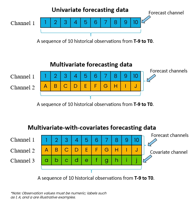
Univariate forecasting data contains only a single channel observed over time. The forecasting model relies solely on the historical values of the forecast channel.
Multivariate forecasting data contains multiple forecast channels observed over time, where all variables are jointly modeled and forecasted based solely on their own historical values, without additional covariates.
Multivariate-with-covariates forecasting data contains multiple time-dependent channels observed over time, where one or more channels are forecast channels and the remaining channels serve as covariates to improve prediction accuracy.
The forecasting dataset must specify the following:
Number of all available channels.
Forecast channels: which signal channels should be predicted by the forecasting model.
Forecasting strategy:
Recursive forecasting: the model predicts future steps sequentially using previous predictions.
Direct multi-step forecasting: the model predicts all specified horizons in a single model output.
Forecast horizons: how many future time steps the model needs to forecast in one inference. (Fixed to 1 when recursive forecasting is enabled.)
Recursive length (recursive forecasting only): number of recursive prediction iterations performed during training. It should be chosen according to the target forecasting scenario.
Cross-instance mode: enables training a model that generalizes across multiple similar instances (e.g., devices, machines, products) or only a single instance.
When enabled, data files from multiple instances must be imported. The model learns patterns shared across instances.
When disabled, only one data file from a single instance needs to be imported.
The forecasting data transformation for BYOD training:
For forecasting, time series data is automatically transformed into training samples using a sliding window approach. Each sample consists of a lookback window of historical observations from all channels and the corresponding future value(s) to be predicted. During training configuration, users need to specify the following parameters:
Lookback: how many historical observations used as input, and it should be large enough to cover the potentially informative lags. Users can either define this value based on the forecasting scenario or refer to the recommended lookback derived from dataset analysis.
Stride: how many time steps the sliding window advances between samples. Smaller values create more overlapping samples; larger values reduce training set size. (Note that stride applies to the training data conversion only and has no effect during inference.)
The following example illustrates how a univariate time series with 10 observations is transformed into training samples using horizon = 1, lookback = 5, and stride = 1:

Note:
Each continuous data file must contain at least lookback + max(forecast horizons) time steps to generate one training sample. Multiple files are supported, but each file is converted independently and is not merged with other files, preserving the original time order of the data.
Forecasting strategy: recursive forecasting and direct multi-step forecasting
Forecasting supports two prediction strategies: Recursive Forecasting and Direct Multi-Step Forecasting. Understanding the differences between these approaches helps users select the most suitable forecasting configuration.
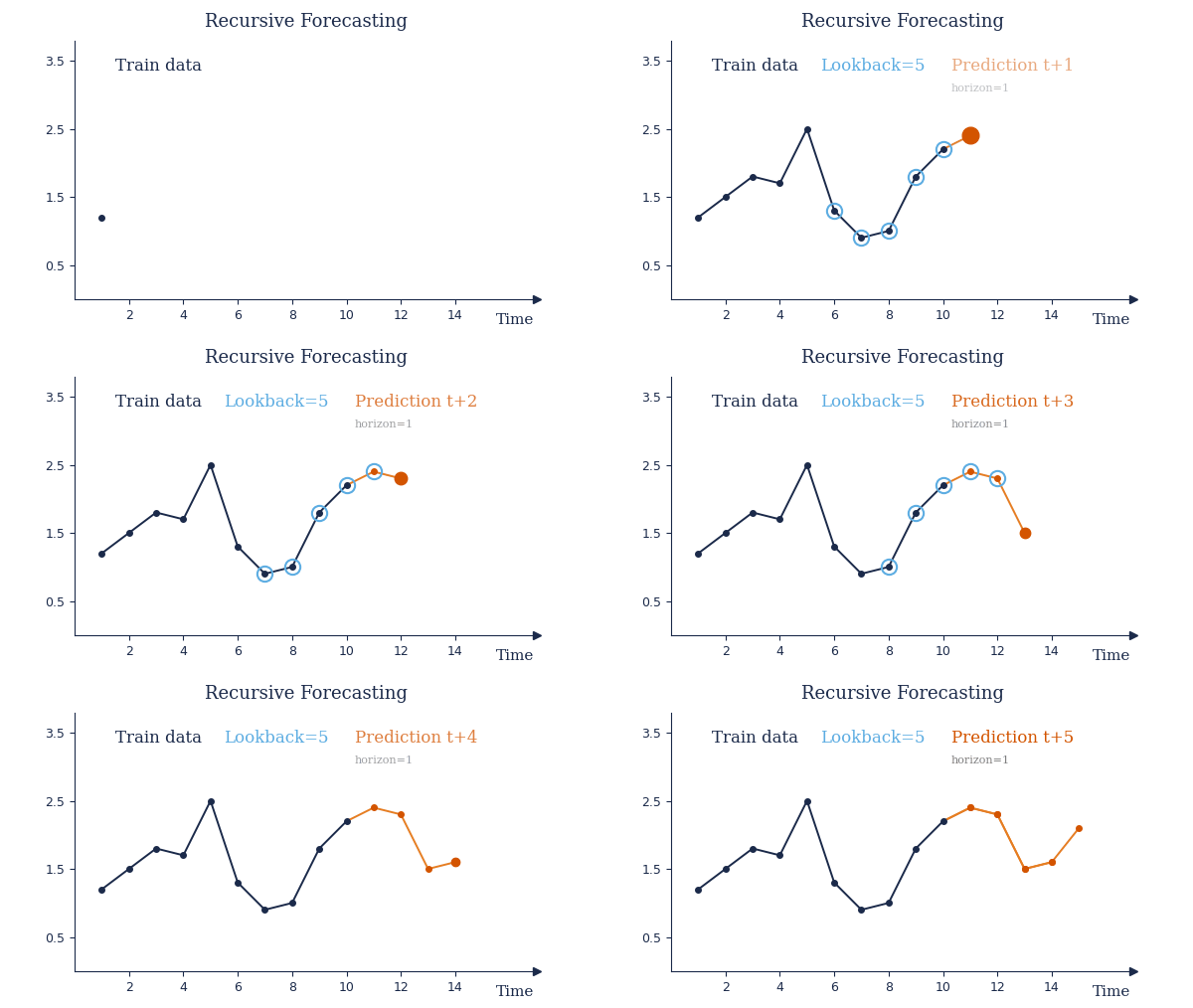
Recursive forecasting predicts one future time step at a time. Each prediction is fed back into the model as input for the next prediction. The forecast horizon is fixed to 1, and longer forecasts are generated recursively over multiple steps.
Requires actual values for all channels only at the first inference. Subsequent forecast steps can use previous predictions for forecast channels, while covariates, if any, must continue to use actual values.
During training, users specify a Recursive Length to define the number of recursive steps used for optimization. During deployment, the actual number of recursive prediction steps is flexible and can be determined based on model performance or application-specific stopping criteria.
Advantages: Flexible forecast length. Suitable for long-range forecasting.
Considerations: Prediction errors may accumulate over multiple recursive steps.
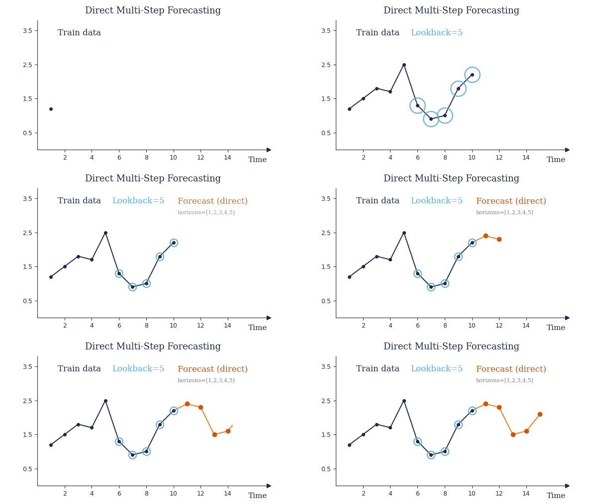
Direct multi-step forecasting predicts multiple future time steps simultaneously in a single model output. Users specify the forecast horizons to be predicted directly.
Requires actual values for all input channels at every inference.
Advantages: No error accumulation across forecast steps. Stable forecasting performance for predefined horizons
Considerations: Forecast horizons must be specified in advance. Less flexible if the forecast length changes.
Forecasting Strategy on Different Time Series Data
Univariate Time Series Forecasting

Multivariate Time Series Forecasting

Multivariate-with-covariates Time Series Forecasting

Data Format Conversion
Based on the description above for the data sample formats for anomaly detection, classification, and regression, you can manually change the data sample format to adapt to different task changes. Here is an example of data format conversion from classification to regression:

Main steps:
Use different classes as target labels.
Add the first column as a target and append a specific class of time-sequential data on the same line.
Make the regression data samples randomly ordered and save them for the regression training task.
Notes:
Currently, there is support for single-class classification only. Converting from classification to regression data format is relatively straightforward. Also, converting from single-target regression data samples to classification is possible. However, you must ensure that the converted labeled classification files are balanced in terms of data samples.