Arc Fault Circuit Interrupter (AFCI) Solution Application​

Introduction

This document describes the NXP DC AFCI solution with edge-based machine learning for real-time arc fault detection and predictive maintenance. It provides an end-to-end workflow covering data acquisition, labeling, model training, evaluation, and deployment on embedded targets.

Background and Motivation

The rapid growth of photovoltaic (PV) and energy storage systems—driven by decarbonization targets and increasing electricity demand—has significantly expanded system scale and complexity. Arc faults (ARC) can occur due to loose connections, cable aging, insulation degradation, or mechanical stress. These faults generate localized high temperatures that may ignite surrounding materials, posing severe safety risks. To address this challenge, the NXP AFCI solution combines:

• High-frequency signal acquisition

• Edge machine learning inference

• Real-time fault detection and diagnostics

Solution Overview

The AFCI solution provides a unified toolchain (TSS) that enables:

• Data logging and visualization

• Data labeling and dataset generation

• Feature extraction and analysis

• Model training and evaluation

• Deployment to embedded devices Additionally, NXP provides a lab environment compliant with UL1699B for reproducible arc fault generation and data collection.

Lab Environment

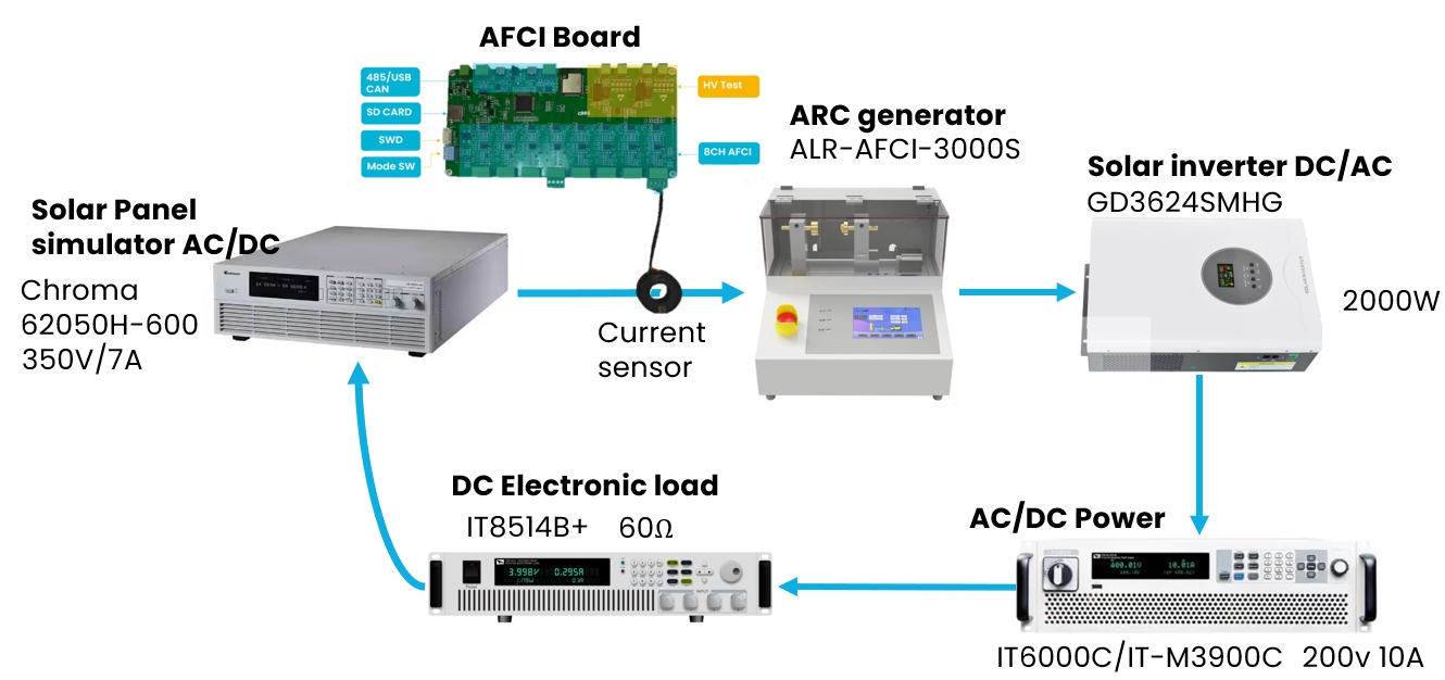
The NXP AFCI Lab setup follows the UL1699B standard and includes:

• ARC generator (ALR-AFCI-3000S)

• Current sensing hardware

• Controlled fault injection capability This setup enables realistic arc fault simulation and high-quality dataset collection.

Data Pipeline

Data Acquisition

Sampling rate: 320 kHz by default, adjustable based on actual ARC signal features Data source: current sensor Data transfer: USB to TSS tool The AFCI board streams high-frequency current data for real-time monitoring and offline processing.

Project configuration

Key configuration parameters:

• Target board (or equivalent CPU)

• Number of classes (e.g., 2 classes: ARC vs Normal)

• Sampling rate (must match acquisition rate)

• Memory constraints (RAM/Flash)

• Sensor type and channel configuration

Step by step:

1. Navigate to AFCI domain from left menu bar.

2. Select Create from navigation bar.

3. Click the AutoML Project button and create a project.

4. Configure the project settings.

   a. Choose your target board. If the real board is not in the list, choose a board with the same CPU.

   b. Set the number of classes according to the dataset and your requirements. We use 2 classes as an example.

   c. Set the sample rate based on the data collection sampling rate. In this case, set it to 320000 Hz (320 kHz) to match the AFCI board’s sampling rate.

   d. Set Library Max RAM and Library Max Flash for the library according to your actual situation. Keep default values for this example.

   e. Configure the sensor type and the number of channels assigned to each sensor based on the uploaded data. Click the + Add button to save the configuration of the current sensor. In this sample, a Current sensor with 1 channel is used.

   f. Confirm completion of the creation. After successful creation, it appears as a working project in the project list.

Data logging

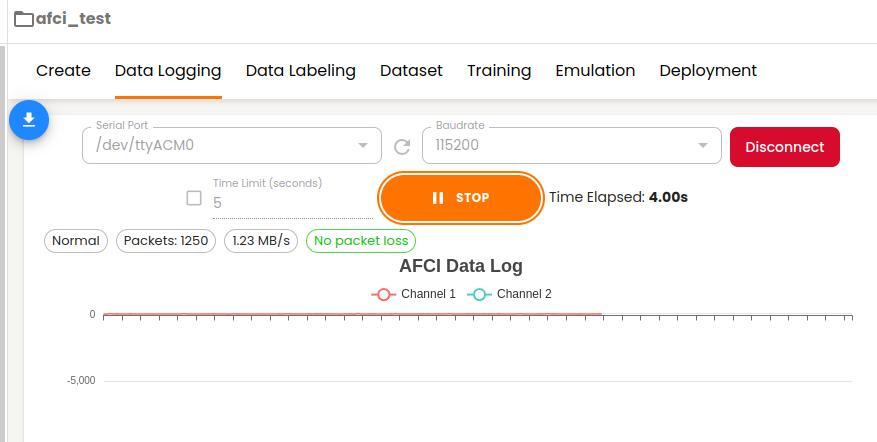
After project creation, TSS automatically guides users to Data Logging panel. Then follow the steps below:

1. Board connection as follows:

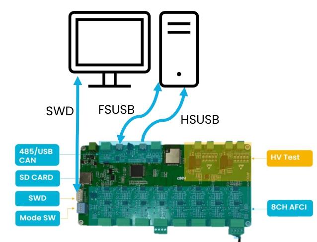
SWD is used for firmware programming and debugging. Connect the SWD pins (SWDIO and SWCLK) to your debugger/programmer device. HSUSB connection is used for data logging and communication with TSS. FSUSB connection is used for logs output and shell commands input. Connect the USB ports on the AFCI board to your PC using a standard USB cable.

2. Download AFCI FW project and flash the FW onto AFCI board.

3. Set SW1 to On Off Off Off to enable data logging mode. More details about AFCI FW usage, please refer to AFCI FW User Guide.

4. Connect AFCI board to PC via USB cable.

5. Select serial port and open it.

6. Start data logging by clicking the Start button.

7. Click Stop button to complete data logging when sufficient data is collected.

Data Labeling

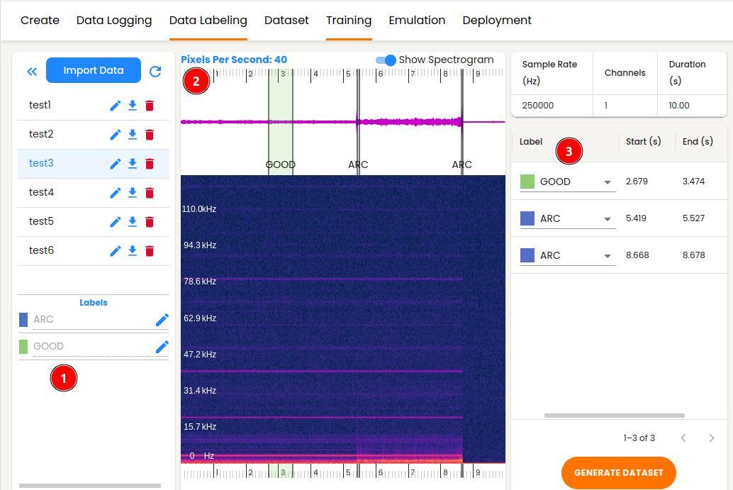
The Data Labeling function enables users to categorize the imported raw data by applying corresponding tags, such as ARC and Normal, to different sections of the current graph through a visual interface. The TSS segments the raw data based on labels and creates datasets optimized for training machine learning models. Users need to complete the following steps:

1. Give a friendly name for different classes (optional).

2. Drag mouse to select one data segment on the waveform graph to be used for labeling.

3. Select the label for corresponding data segment from the label list on the right side of window.

4. Repeat step 2 and step 3 to complete all the data labeling.

Dataset Generation and Feature Engineering

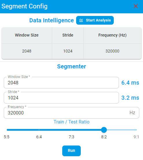
Segmenter Configuration

Click the GENERATE DATASET button. Fill the training window size, stride and frequency based on the dataset features. Recommendation: Use Data Intelligence for automated parameter suggestions.

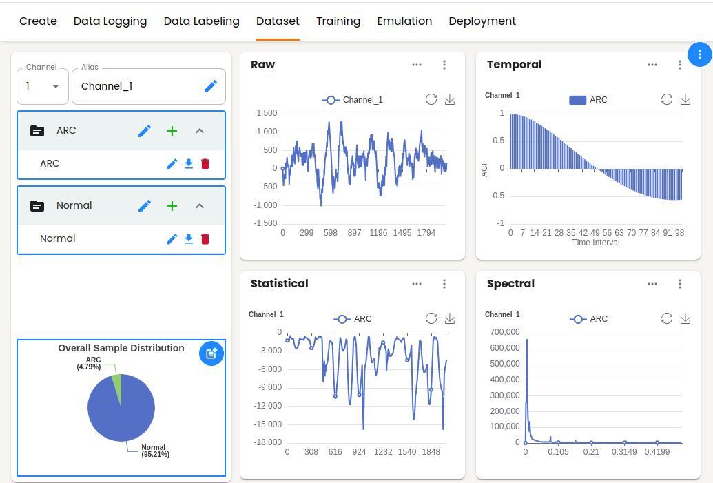
Dataset

After completing the data generation, the user will be automatically guided to Dataset panel. All training data generated by Segment from Data Labeling have been automatically imported. You can view the distributions of the dataset across different domains on this page as visual graphs.

Data feature chart can be viewed with single file or multiple files in different domains. This feature can facilitate users to analyze and compare intuitively.

In this page, TSS also supports users importing other datasets in CSV or wav format by clicking + button in every label group.

• Raw domain with Combined and Separated modes.

• Temporal domain with the ACF and the PACF operators.

• Statistical domain with the Min, Max, Mean, Mean_Plus_STD and Mean_Minus_STD operators.

• Spectral domain with the FFT, STFT and Cepstrum operators.

Training

The AFCI solution is built on Machine Learning Classification task. For the detailed training process, please refer to the Training chapter.

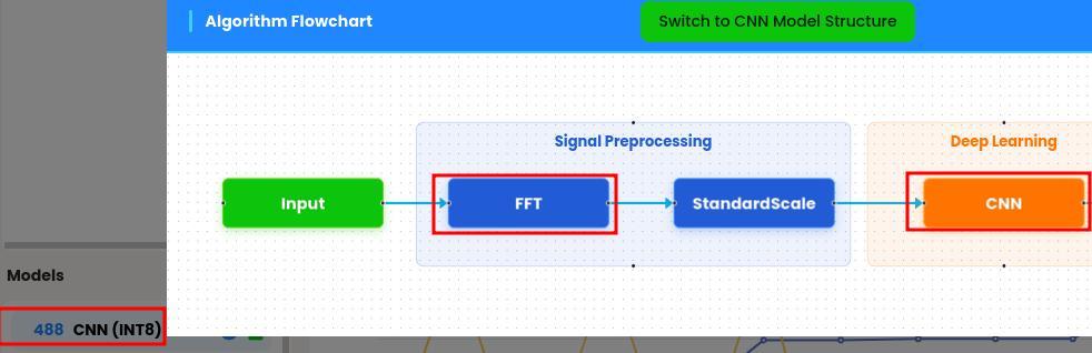
The MCU chip MCXN547 integrates Power Quad and Neutron hardware IPs. The TSS tool efficiently leverages Power Quad to speed up FFT calculation in signal process pipeline, and quantized DL models in prediction.

For model selection, if model benchmark is comparable, prioritize using the algorithm with FFT.

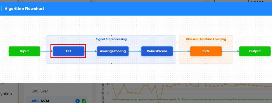
For DL models, prioritize using the ones optimized for int8.

Emulation

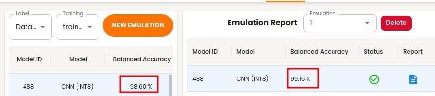
The TSS emulation feature provides a rich set of functions for evaluating trained models. Please refer to the Emulation chapter for detailed description of emulation.

Users need to validate model performance prior to deployment. Emulation accuracy should closely match training accuracy result. A significant drop indicates potential overfitting.

Deployment

The TSS deployment feature provides flexible options for library or binary generation. Please refer to the Deployment chapter to learn more about the deployment process.

Algorithm Library

Linked into application firmware Requires recompilation for updates

Algorithm Binary

Self-contained executable Can be flashed independently Enables runtime algorithm upgrades without rebuilding the application

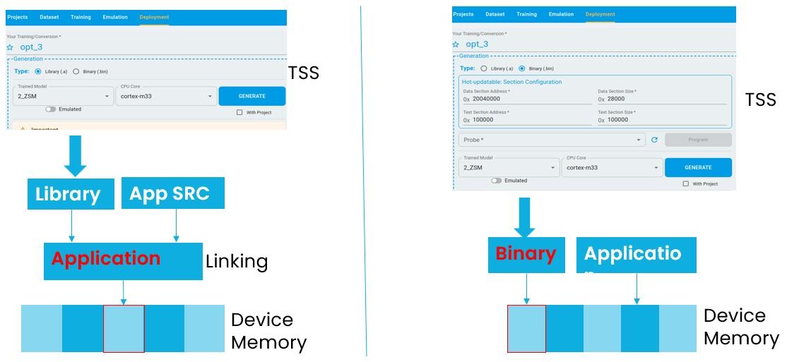
Library vs Binary

Traditionally users select one library and link it into device application, and then flash the application onto device for evaluation. If users would like to evaluate multiple algorithm libraries, they have to repeatedly execute the linking operation, which should be time-consuming for large projects.

Key Differences

Aspect	Library	Binary
Integration	Compile-time	Runtime
Update method	Rebuild firmware	Flash binary only
Flexibility	Low	High

Binary Requirements

• Define flash and RAM regions explicitly

• Flash binary to specified memory location

The generation process differences between algorithm library and binary

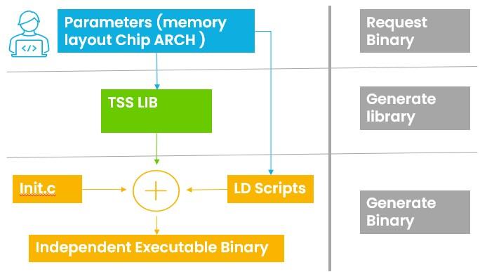
The algorithm is self-contained, which does not rely on any external symbols. After flashing the algorithm binary onto an independent section, the application can invoke algorithm APIs in runtime. Users can only flash the algorithm binary without reflashing application code.

The algorithm binary is generated based on the algorithm library. We implemented an application entry and a linker script. We leveraged the ARM GCC toolchain to link the algorithm library into an independent and executable binary.

The differences between algorithm library and binary usage

1. During generating binary, users need to specify both the flash and RAM start address and size separately.

2. Need to flash the binary onto the address specified by step 1

The differences between algorithm library and binary runtime Integration

The TSS tool provides a unified interface for algorithm library and binary in timeseries.h.

typedef struct tss_task_ops
{
    int task;
    union
    {
        tss_ad_task_ops_t ad_ops;
        tss_ad_odl_task_ops_t ad_odl_ops;
        tss_cls_task_ops_t cls_ops;
        tss_oc_task_ops_t oc_ops;
        tss_reg_task_ops_t reg_ops;
    };
    const tss_algo_attribute_t *(*algo_attribute)(void);

} tss_task_ops_t;

If linking algorithm library into application, need to invoke the API of tss_get_task_ops to get the instance of tss_task_ops_t.

If users use the algorithm binary, need to retrieve the API of tss_get_task_ops address from the binary header and invoke it.

Please read the more details from the example project.

#ifdef ENABLE_BINARY_ALGO
    tss_binary_header_t* (*entry)(void);
    extern uint32_t __base_BINARY_TEXT;

    if (*(uint32_t *)((uint32_t)(&__base_BINARY_TEXT) + 1) == BLANK_BINARY_ENTRY)
    {
        return -1;
    }
    // Convert integer address to function pointer
    entry = (tss_binary_header_t* (*)(void))(uintptr_t)((uint32_t)(&__base_BINARY_TEXT) + 1);
    tss_binary_header_t *p_algo_head = entry();
    PRINTF("MAGIC NUMBER:");
    int i = 0;
    for(i = 0; i < 8; i++)
    {
        PRINTF("%c", p_algo_head->magic[i]);
    }
    PRINTF("\r\n");
    p_task_ops = p_algo_head->get_task_ops();
#else
    PRINTF("\r\nStatic library model is using...\r\n");
    p_task_ops = tss_get_task_ops();
#endif

Summary

The NXP AFCI solution delivers a complete edge AI pipeline for arc fault detection, combining:

• High-frequency sensing

• Advanced signal processing

• Efficient ML deployment It enables robust, real-time protection in modern electrical systems.