Dataset
The dataset is used to import user signal data for time series projects, including data validity checking and data visualization.
Data Import
Import user training data into the project.
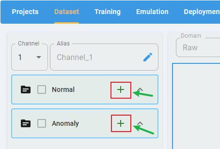
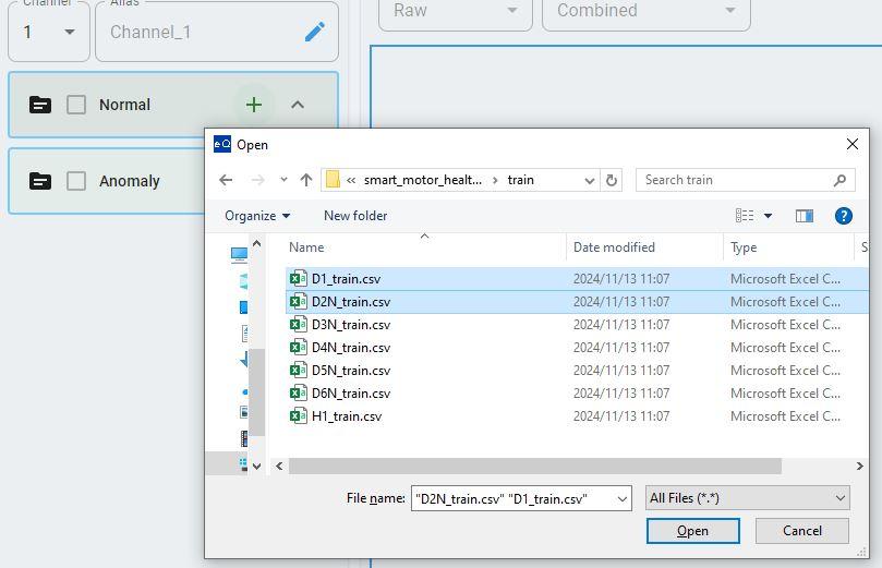
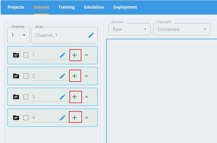
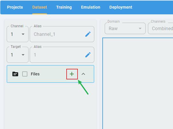
In any type of project, click the + button to open the file selection dialog.
Select the files to load. The data loader supports the selection of multiple files at one time.
Data Preview
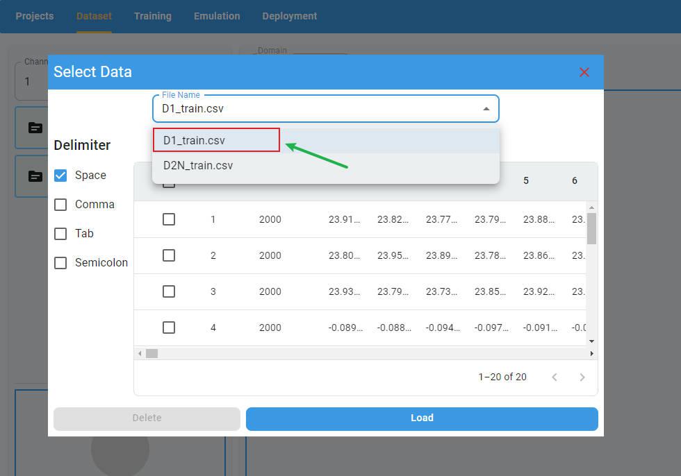
After selecting the data files, the preview screen appears with the delimiter selection panel on the left and the data display panel on the right.
The default delimiter is space. If any other delimiter is used, select option 1 in the delimiter selection panel.
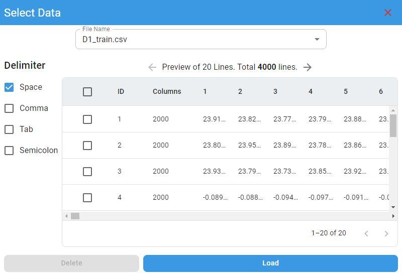
If you have more than one file loaded at the same time, you can select the file you want to preview from the file list.
If you want to delete rows in the preview panel, select the rows to delete and click the Delete button. The selected rows will be deleted.
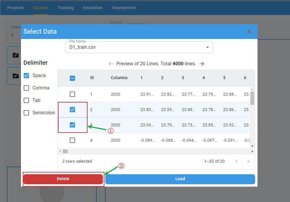
To load the data files in the preview panel, click the Load button. All imported files are loaded and the files are displayed in the list of imported files.
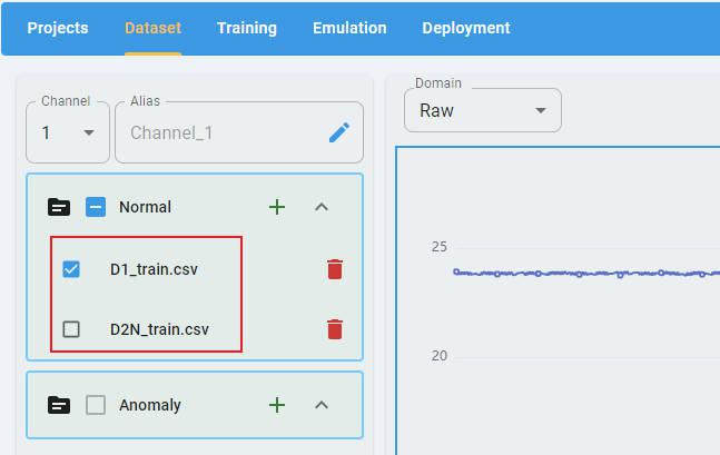
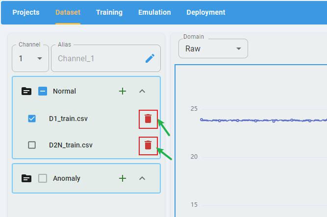
You can click the buttons beside the filename to delete the imported file.
Rename the Channel Names
By default, the label of each channel is “channel” + index, such as “Channel-1”, “Channel-2”.
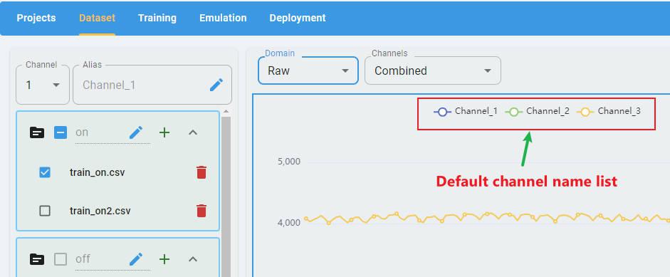
You can edit the alias of the channels to create new channel labels (optional).
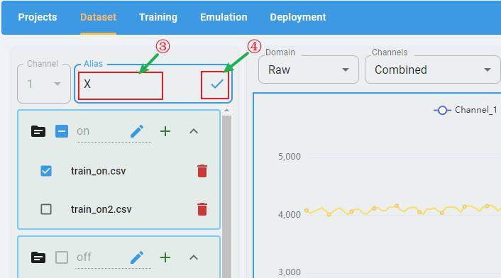
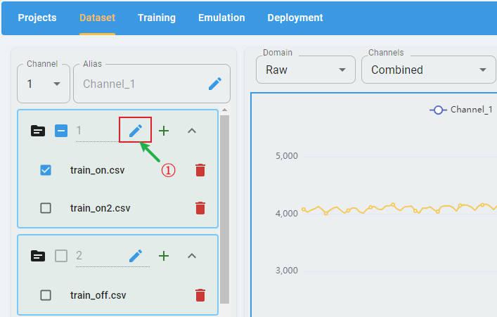
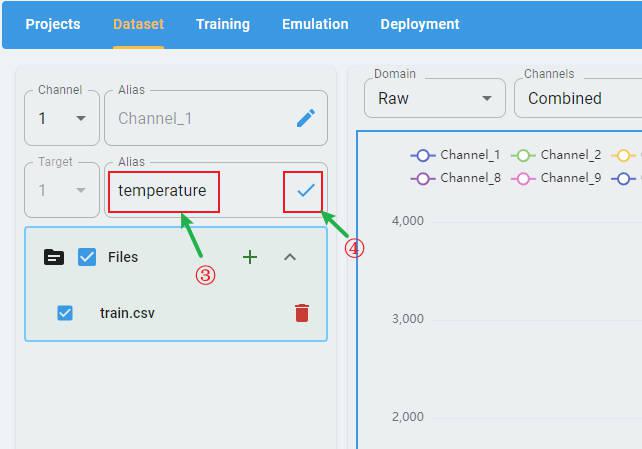
To edit the alias, first select a channel in the channel list, then click the edit button:
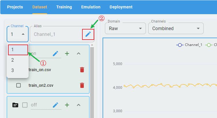
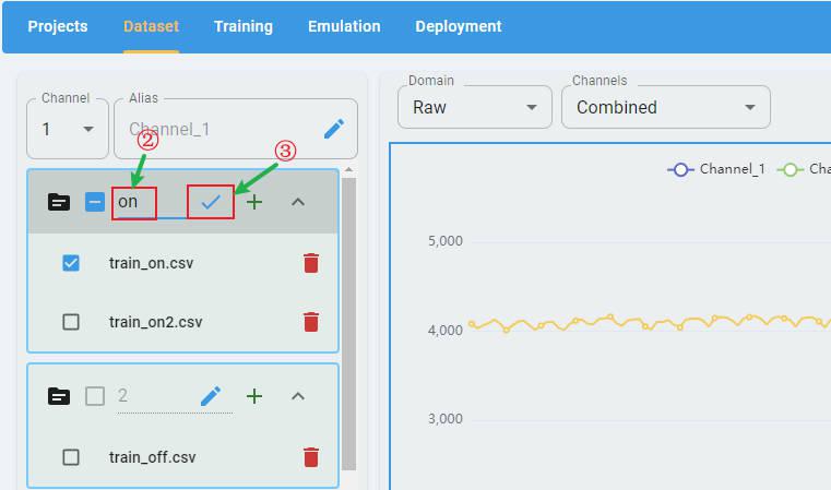
Input the new channel name. Click the check button to apply the rename.
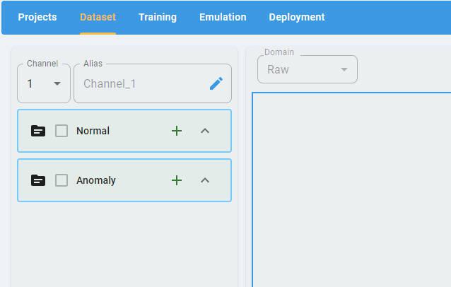
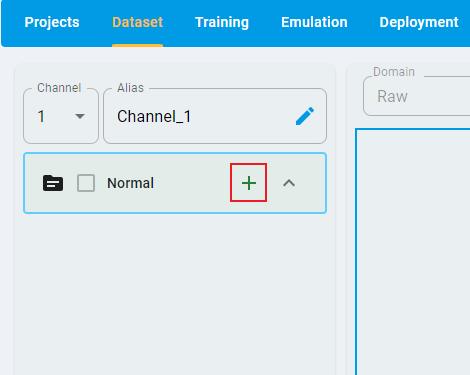
Anomaly Detection
For an Anomaly Detection project, there are two classes of data files that must be imported: Normal and Anomaly. Each class must have at least one data file loaded.
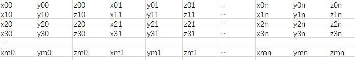
Data file format: One sample per row, containing all channels, with samples separated by delimiters (space, comma, tab, and semicolon). Here is a data file example that contains m samples with n values × 3 channels (x, y, and z). The channel is the last dimension.
n-Class Classification
For an n-Class Classification project, n (n≥2) classes of data files must be imported. Each class must have at least one data file loaded.
Data file format: One sample per row, containing all channels, with samples separated by delimiters (space, comma, tab, and semicolon). Here is a data file example that contains m samples with n values × 3 channels (x, y, and z). The channel is the last dimension and uses the same format as Anomaly Detection.
Click the + button and load the data files for all classes.
By default, the label of each class is a class index. You can edit the alias of the class to create a new class label (optional).
To edit the alias, first click the edit button:
Second, input the alias string, then click the check button to apply the rename.
1-Class Classification
For a 1-Class Classification project, only one class of data files is imported, which represents the positive class.
The file format is the same as Anomaly Detection and n-Class Classification.
Regression
The prediction targets of a regression project are continuous values. Therefore, you can put all data into one file (or split it into multiple files with no categories).
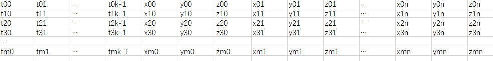
Data file format: One sample per row, containing all channels, with samples separated by delimiters (space, comma, tab, and semicolon). The first k columns (k is the target number, which is set when the regression project is created, k ≥ 1) are the target values to predict. Here is a data file example that contains m samples with n values × 3 channels (X, Y, and Z), and k targets.
You can provide an alias for the target name for clarity (optional).
Select the target that you want to rename and click the edit button.
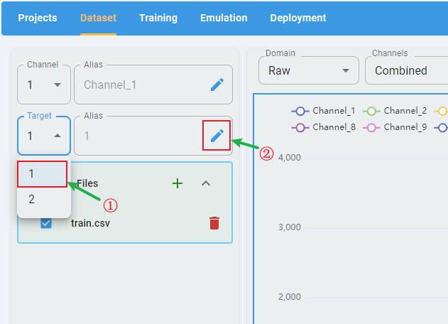
Input a new target name and click the check button to apply the rename.
Data Visualization
After the data files have been configured and loaded, the data preview screen appears. The graph of the data file appears in the right panel.
A data visualization toolset is provided, which enables users to view the distribution of data in raw, temporal, statistical, and spectral domains.
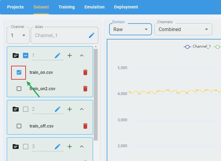
Select one or several files (all operators support multiple files except raw) from the file list to display:
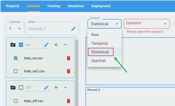
Select a domain:
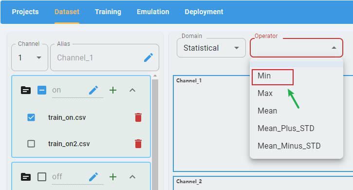
Select an operator:
Note: In Data Visualization, if data has multiple channels, the graph for each channel is plotted separately (except for the raw operator).
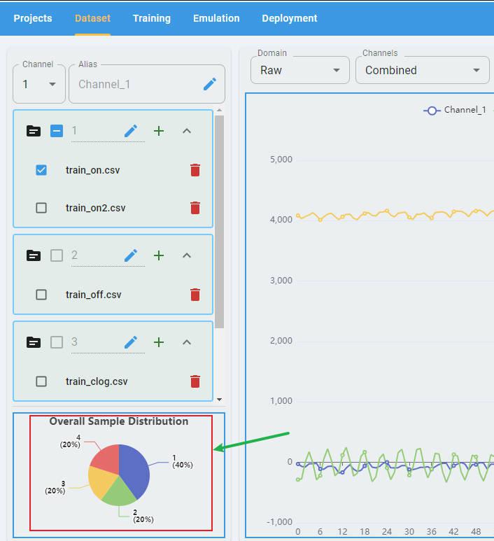
You can click the full screen button to display the graph in full screen mode (optional).
Overall Sample Distribution
The overall sample distribution graph shows the distribution of labels for all the data in the project, which allows users to analyze the data balance.
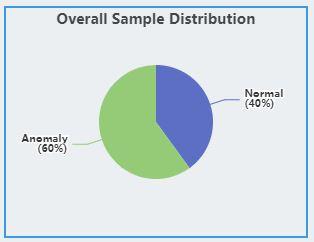
Anomaly Detection
The graph shows the distribution of Normal samples and Anomaly samples.
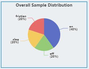
Classification
The graph shows the distribution of all classes.
Regression
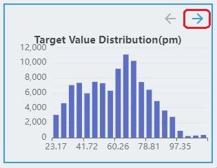
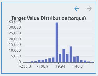
The labels of the regression task are continuous values. Therefore, the distribution of labels is discretized and displayed as a histogram, where the x-axis represents the target value and the y-axis represents the number of samples in the interval.
The regression task supports multiple targets. If the dataset contains multiple targets, click the direction arrow button to see the distribution of other targets.
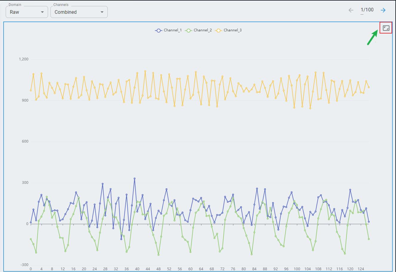
Raw Data
Here is an example of fan state classification data input with only three channels of acceleration data.
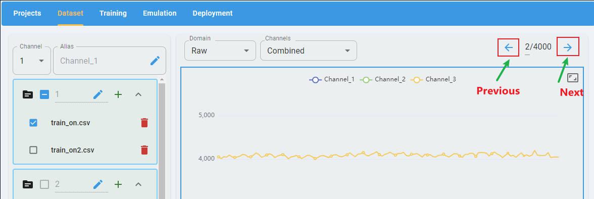
What information is included?
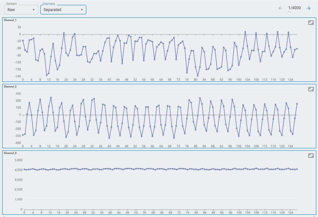
The x-axis represents the time step index. You can see that each data window contains 3 × 128 data points.
The y-axis represents the value of each data point. Multiple channels are rescaled to fit within a data range.
The chart contains only one channel; if more channels are loaded, each channel displays in a different color.
In the top-right corner, there are data forward/backward buttons for quick navigation and data checking.
View selection
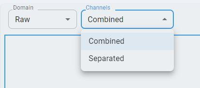
Combined view: data from all channels are plotted on a single graph.
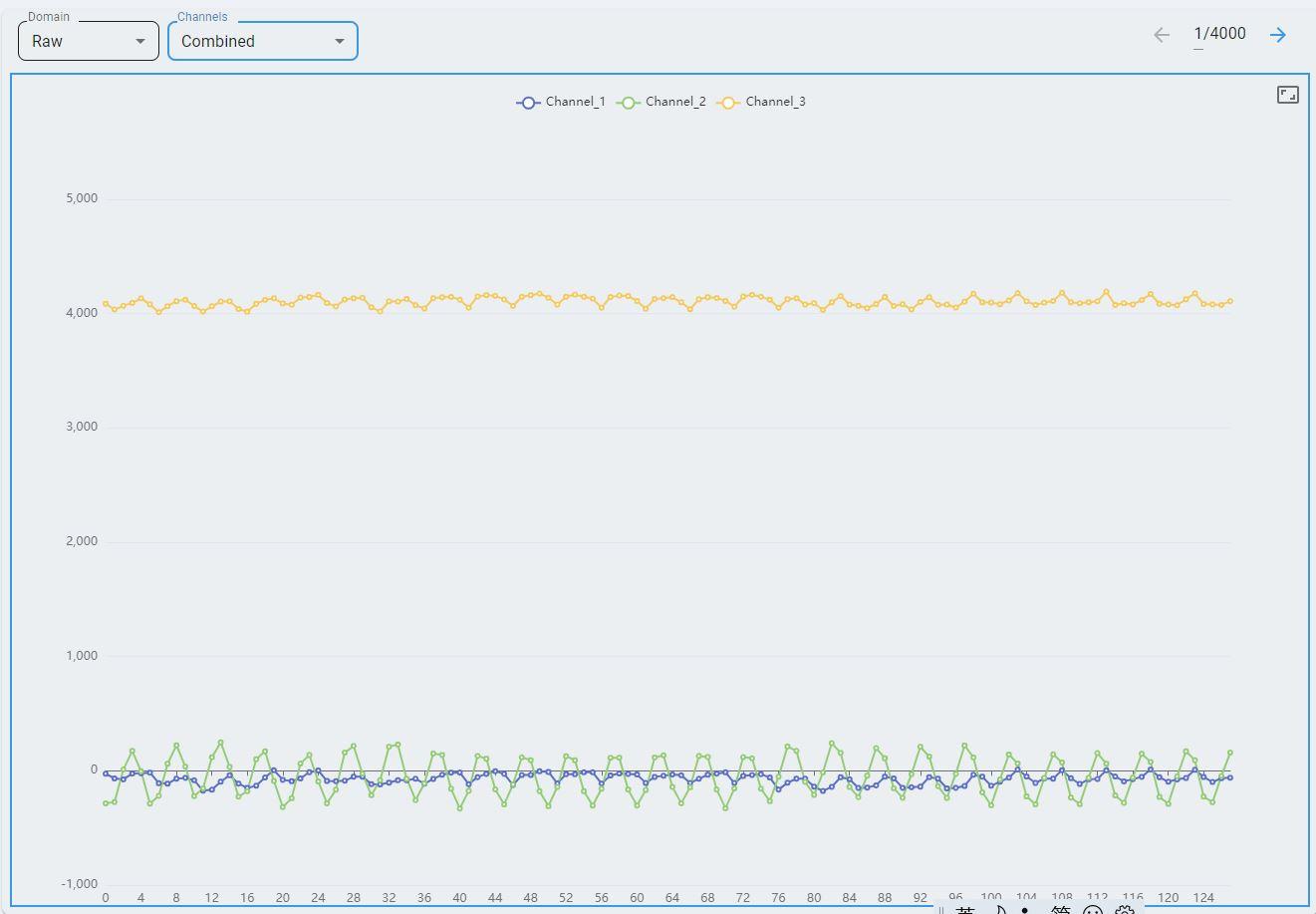
Separated view: data from each channel is plotted on a separate graph.
Temporal Domain
Here is an example of an accelerometer with three channels of data for x-, y-, and z-axis. The following is an overview of the temporal domain.
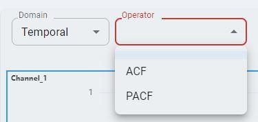
Autocorrelation Function (ACF) is a statistical tool used to measure and analyze how a signal correlates with itself over different time intervals. It provides insights into how a dataset varies with itself at different lags.
Partial Autocorrelation Function (PACF) measures the correlation between a time series and its own lagged values, controlling for the values of the intervening lags. This function is crucial for identifying the order of an autoregressive model. The function helps distinguish the direct relationships between observations at different time points without interference from other lags.
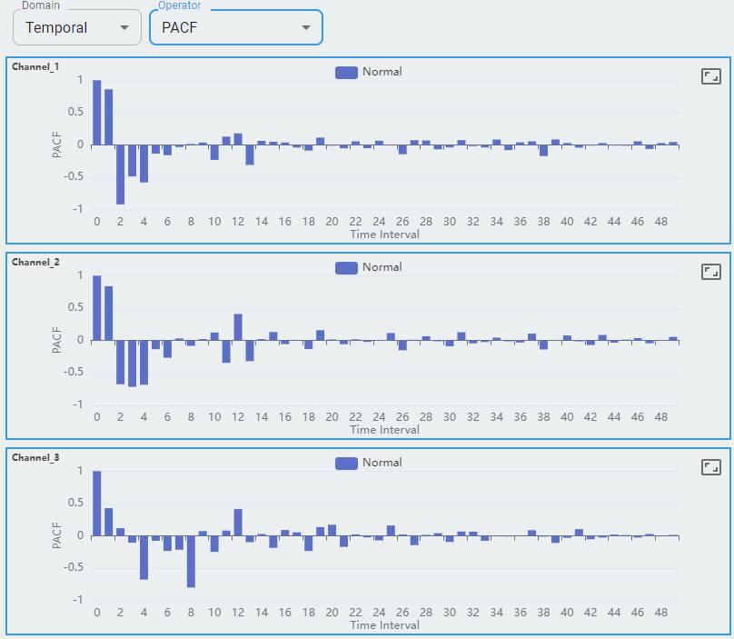
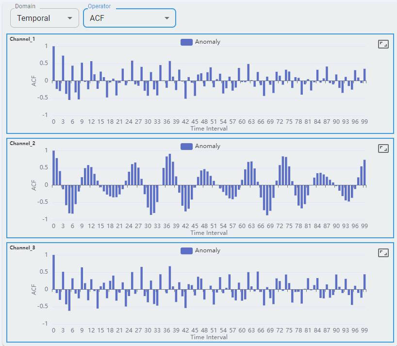
What information is included?
Three channels of the X, Y, and Z axes are shown as channel-0, channel-1, and channel-2.
A maximum of 80 windows of sample data are shown. Each point represents the extracted feature from the temporal domain.
For the temporal domain, ACF and PACF are shown for reference.
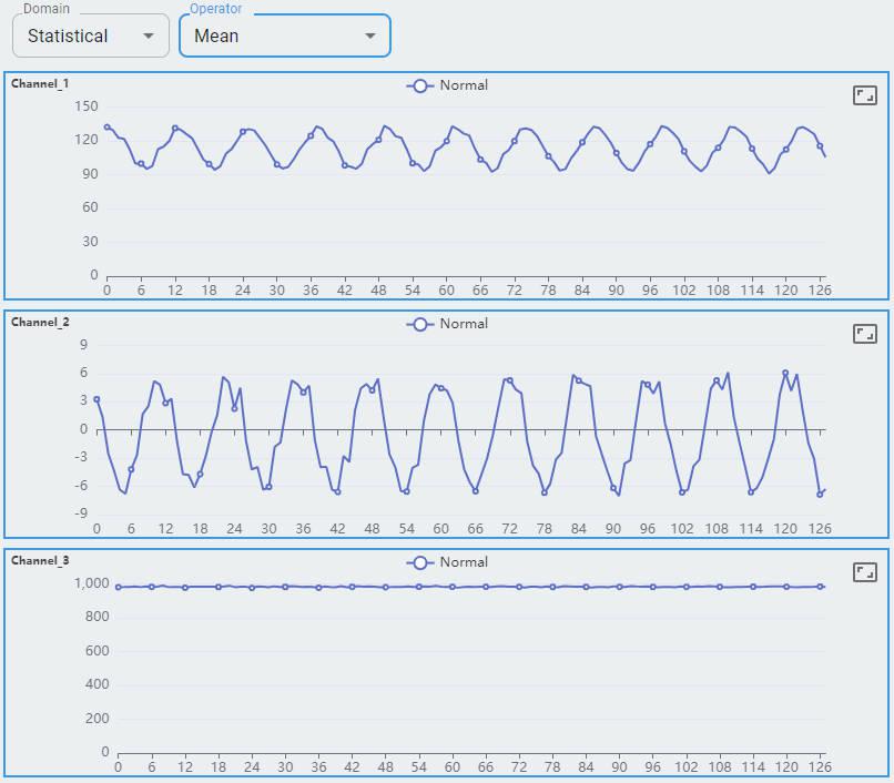
Statistical Domain
Here is an example of an accelerometer with three channels. The window size of the data is 128×3=384, and the sample frequency is 10 kHz. It has 80 windows of data. The following is an overview of the statistical domain.
There are five statistical operators. To plot the graph, select any one from the list.
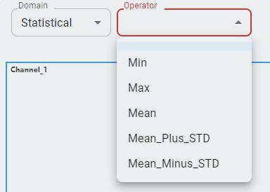
Min
Max
Mean
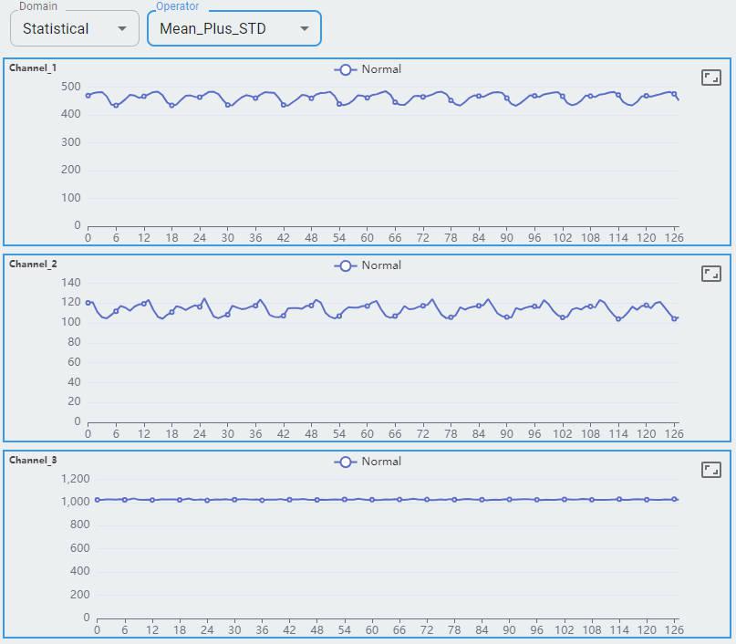
Mean Plus STD
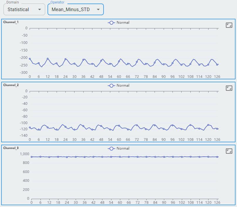
Mean Minus STD
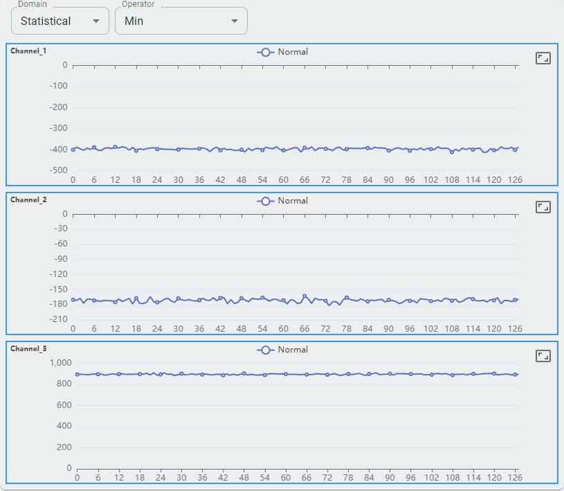
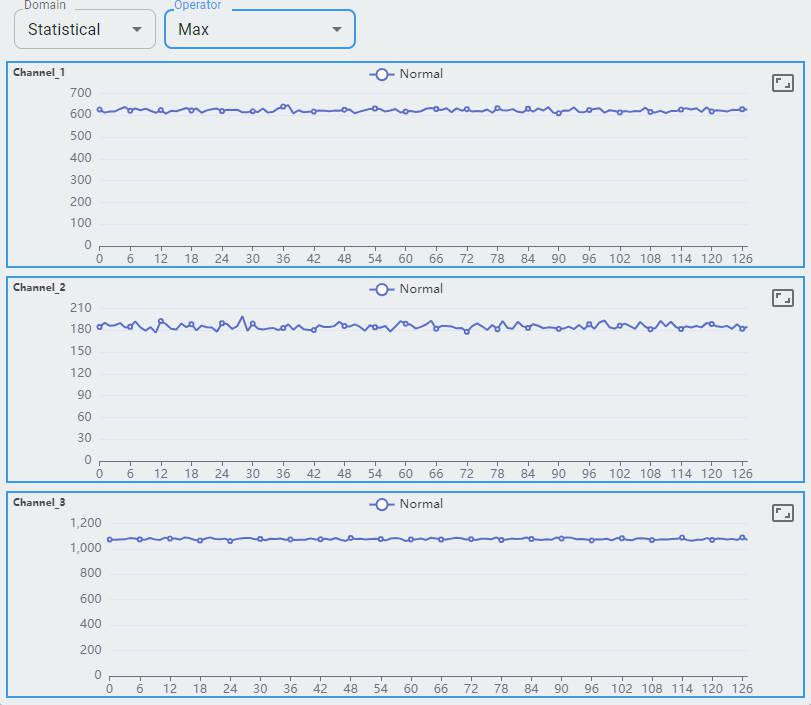
What information is included?
Three channels of the accelerometer are shown as channel-0, channel-1, and channel-2.
Each channel shows 128 feature sets. Each feature set contains a value for min, max, mean, mean plus std, and mean minus std.
The statistical domain shows min, mean, and max for reference. You can expect more support in future releases.
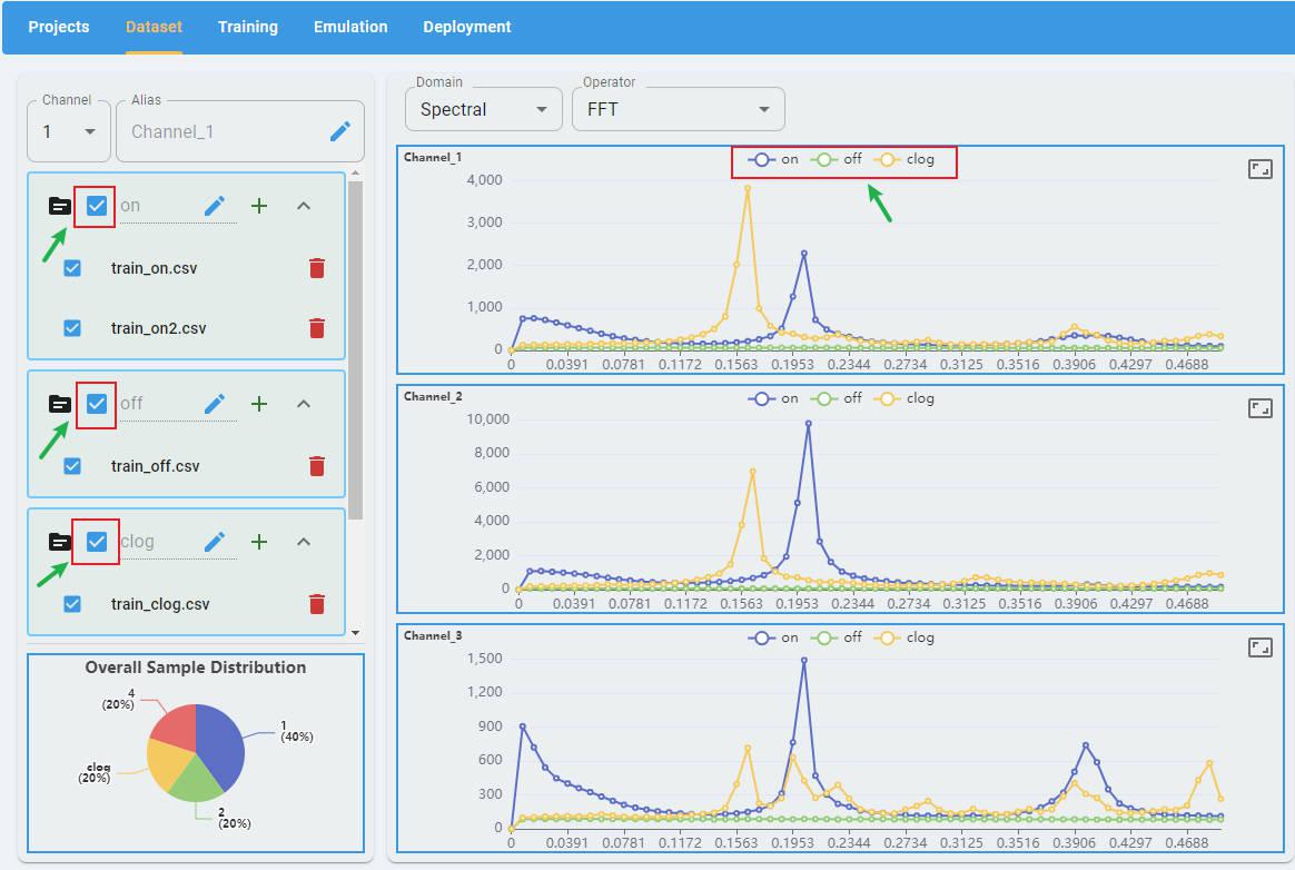
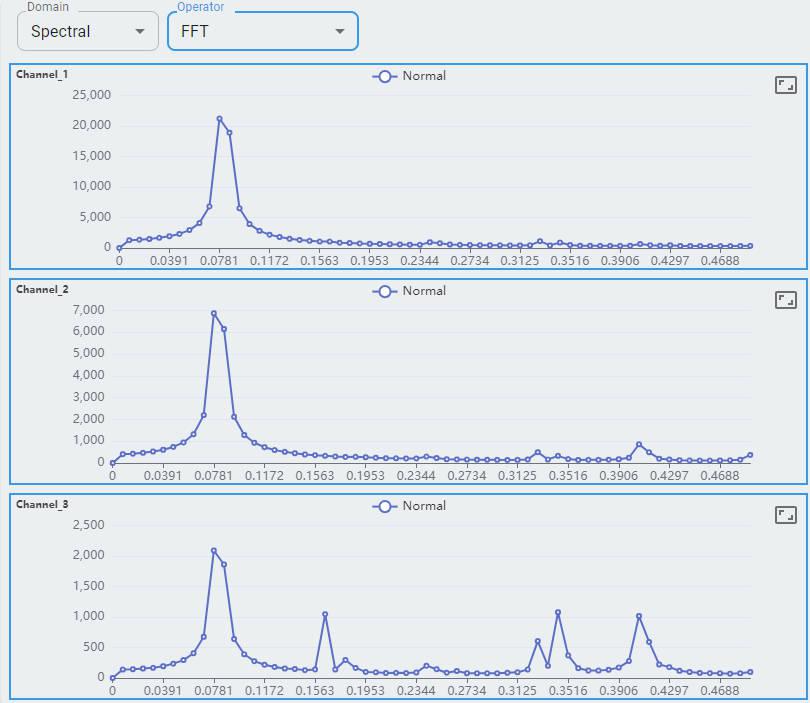
Spectral Domain
Here is an example of an accelerometer with three channels. The window size of the data is 128×3=384, and the sample frequency is 10 kHz. It has 80 windows of data. This is an overview of the spectral domain.
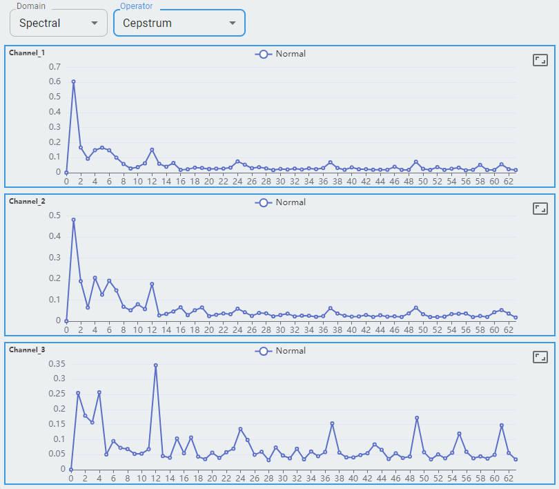
There are three spectral operators. To plot the graph, select any one from the list.
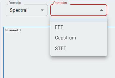
Fast Fourier Transform (FFT) is an efficient algorithm to compute the Discrete Fourier Transform (DFT) and its inverse, drastically reducing the computational complexity from O(N²) to O(N log N).
Cepstrum is the inverse Fourier transform (IFT) of the logarithm of the estimated signal spectrum.
Short-Time Fourier Transform (STFT) is an extension of FFT that computes the Fourier Transform of short, overlapping segments of a signal over time.
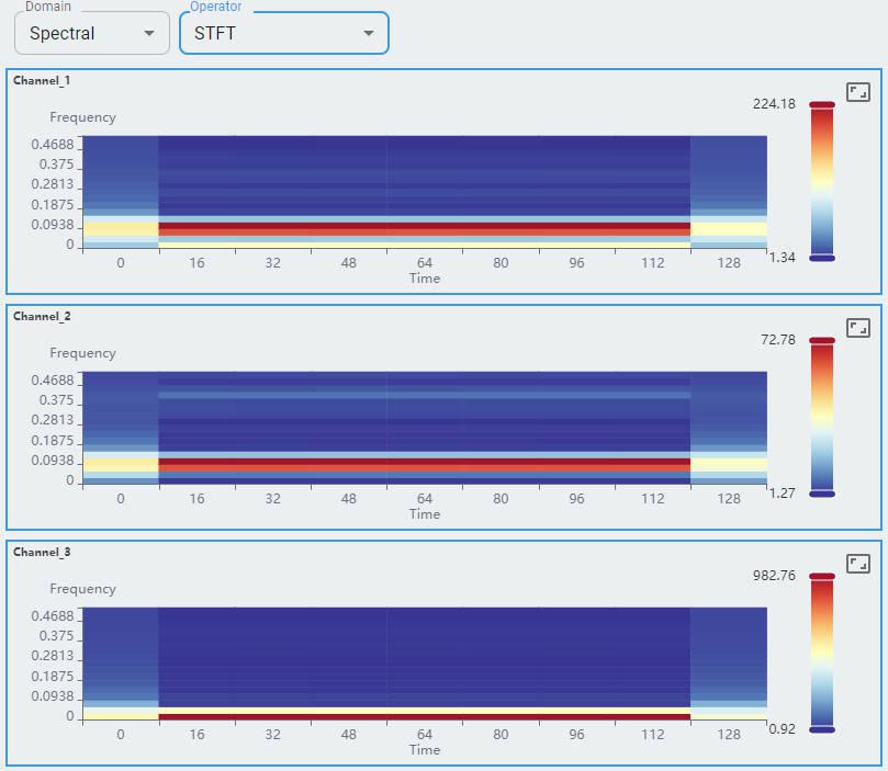
What information is included?
Three channels of the accelerometer are shown as channel-0, channel-1, and channel-2.
Each channel shows its frequency as the x-axis from 0 to 0.5 and the y-axis as its amplitude.
For the spectral domain, FFT (Fast Fourier Transform), Cepstrum, and STFT are shown for reference. More will be supported in the future.
Multiclass Compare
You can select multiple data classes in one view to compare the differences between data classes (STFT and Raw are not supported). Graphs for different classes are plotted on the same graph with different colors. You can toggle the display by clicking the class labels at the top of the graph.