Training
Switch to the Training tab after loading the datasets. The training function is the core technology, including data preprocessing, automation for algorithm hyperparameter searching, benchmark testing, and optimal accuracy fitting optimization for limited flash and RAM size. Model performance can also be evaluated through various benchmark indicators.
Function Layout
The following figure shows the layout of the Training tab, which is divided into three sections:
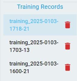
The left frame shows all records of the training.
The middle frame shows the configuration information and optimization process of the specified training.
The right frame shows the benchmark results of the validation set for the specified model.
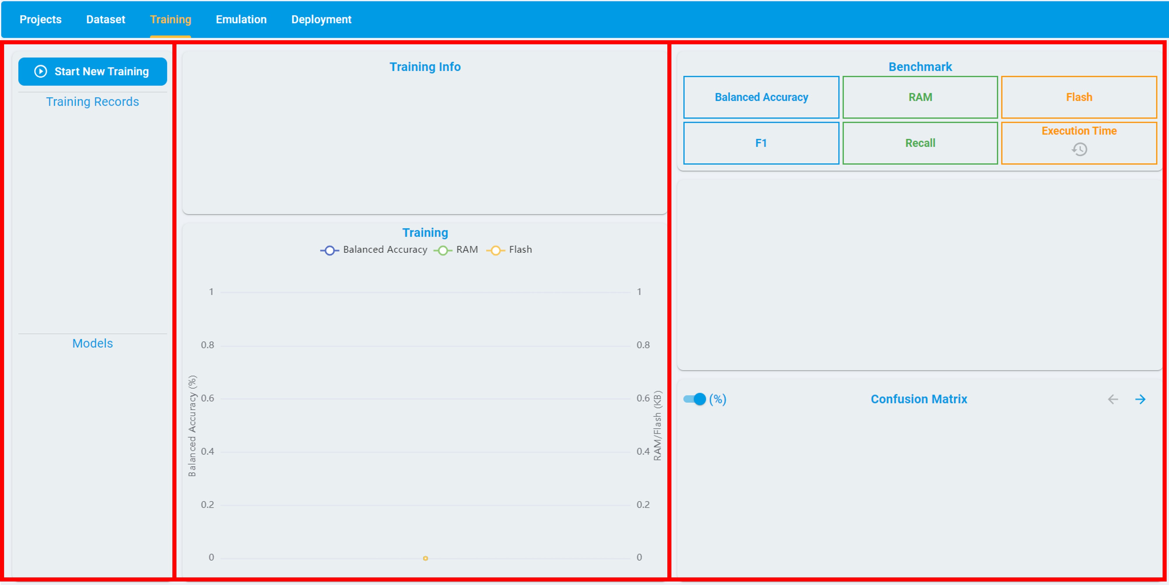
The left frame consists of two parts: Training Records and Models. The Training Records part records all the training tasks created by the user, while the Models part records all the models generated from a specific training task. The models are sorted in descending order of their score. The score depends on the size of RAM/flash usage and some common evaluation metrics for benchmarks.
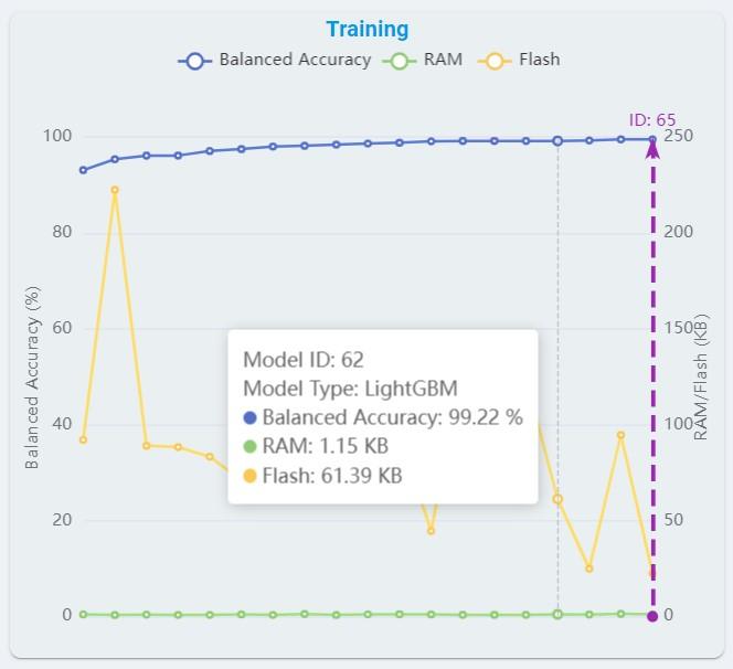
The middle frame consists of two parts: Training Info and Training. The Training Info records the training time, progress, and configuration information; including date, version, model type, max RAM, max flash, quick search, on-Device learn (for anomaly detection), train/validation ratio and data used for training. The Training records the change curves of balanced accuracy, flash, and RAM used with auto machine learning. The same horizontal axis represents the balanced accuracy, flash, and RAM used of the specific model.
In general, there are four types of tasks that support time series-based dataset applications, which are anomaly detection, n-class classification, 1-class classification, and regression. The information in the right frame varies with different task types. The task types are introduced in detail in the subsequent content.
Anomaly Detection
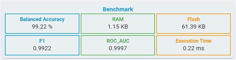
Algorithm Benchmark:
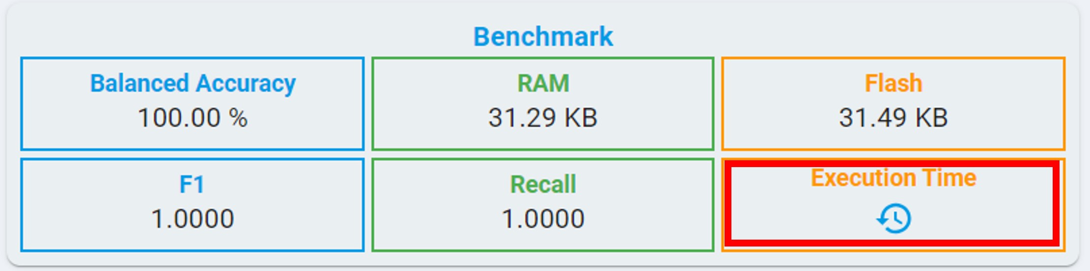
BALANCED ACCURACY: Average accuracy is obtained from both the minority and majority classes.
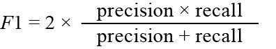
F1: The F1 score is a metric that reflects the global performance of a classifier, the value ranges from 0 to 1.
RECALL: The recall is intuitively the ability of the classifier to find all the positive samples, the value ranging from 0 to 1.

FLASH: Minimum flash size required for selected algorithm.
RAM: Minimum RAM size required for selected algorithm.
Execution Time: The estimated time for one inference in the algorithm library, using the LPC55S36 platform (Cortex-M33, 150 MHz, with hard float-point enabled).
At the same time, you can get the execution time by clicking the clock button.
Algorithm Validation Results:
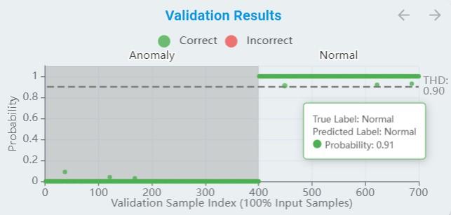
During the training, a part of the data is used for validation from time to time. The training curve reflects those results as the metric of accuracy for the result.
The x-axis means the validation sample index. (For anomaly detection, all samples are used for validation, while classification validates samples according to
Train/Val Ratio.)The y-axis means the probability, which normalized from 0 to 1.
The green points are true positive/negative and the red points are false positive/negative.
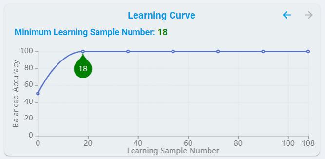
Learning Curve:
For models that support On-Device Learn, learning curves are provided, showing the effect of adding more samples during training.
Confusion Matrix:
For anomaly detection, the confusion matrix table contains normal and anomaly results, see the chart below.
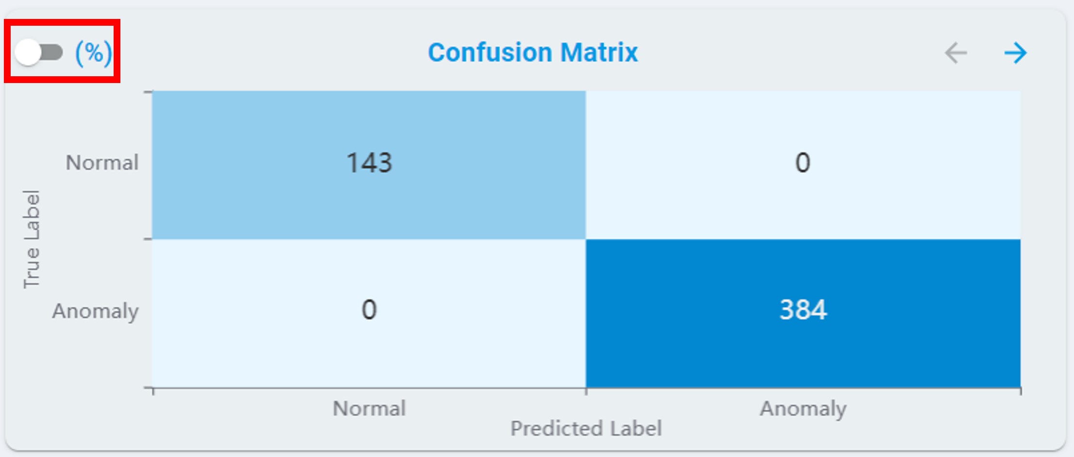
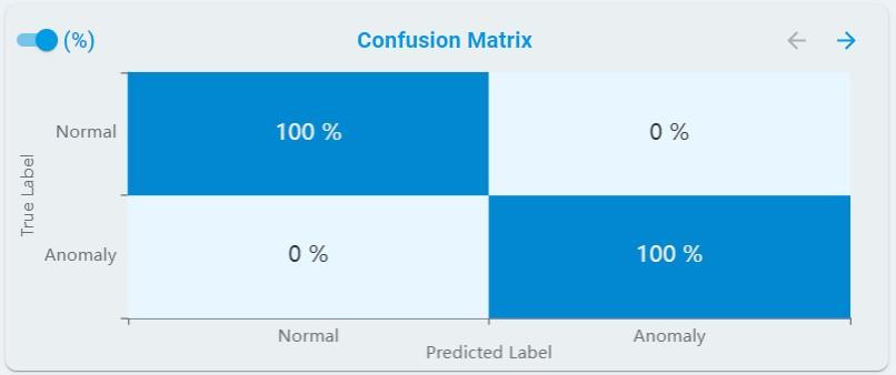
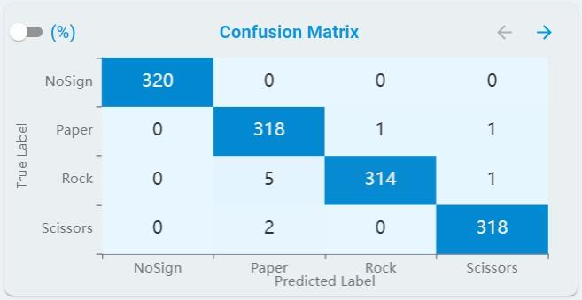
At the same time, you can get the percentage results by clicking the percent(%) button.
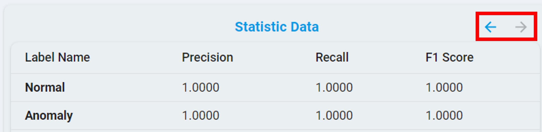
You can also view the statistical results by clicking the arrow button.
n-Class Classification
Algorithm Benchmark:
For classical machine learning in n-class classification tasks, some evaluation metrics are consistent with anomaly detection, such as balanced accuracy, RAM, flash, and F1.
ROC_AUC: ROC_AUC is the area under the receiver operating characteristic curve, the value ranges from 0 to 1.
Unlike classical machine learning, deep learning models quantify the memory requirements using parameters, such as Algorithm Buffer and Model Size.
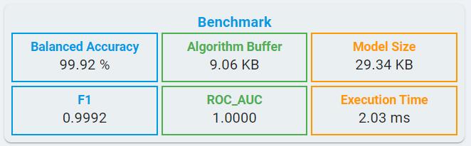
Algorithm Buffer: Buffer estimated for signal processing and inference together.
Model Size: The size of deep learning model for weights and bias.
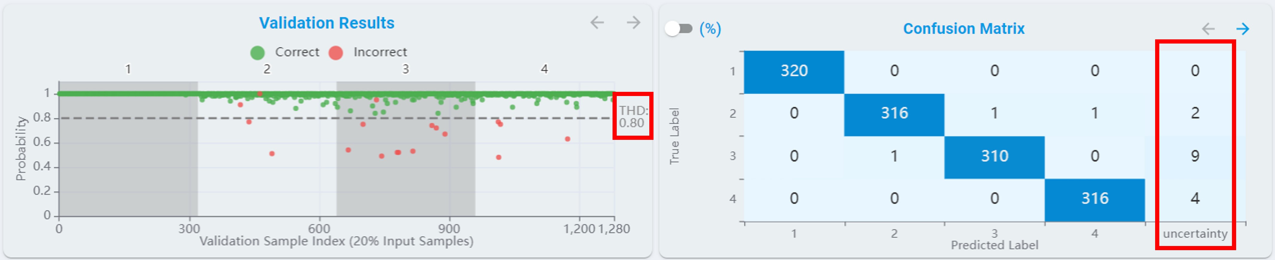
Confusion Matrix:
For n-class classification tasks, the confusion matrix table rescales to fit all classes, see the chart below.
Threshold:
For n-class classification tasks, a Threshold is provided for re-evaluating the performance of the models. The models are reranked according to the balanced accuracy after setting the Threshold.
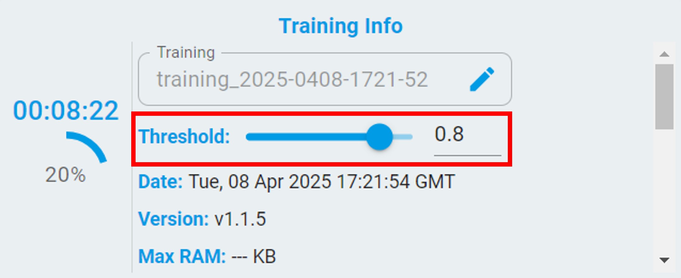
After setting the threshold, a line with the threshold appears in the validation results view. The results with a probability less than the set threshold are re-evaluated as uncertainty.
1-Class Classification
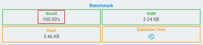
As a special case of classification, 1-class classification only has recall as main evaluation metric because of lack of negative samples.
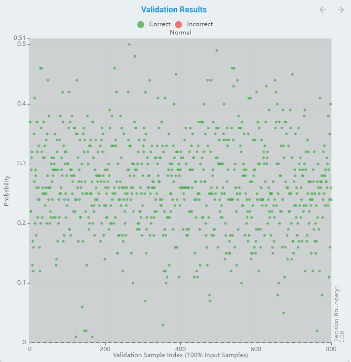
And the validation results chart is not confusion matrix but the distance to decision boundary.
Regression
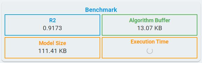
Algorithm Benchmark:
For classical machine learning in regression tasks, benchmark information includes R2, RAM, flash, and Execution time.
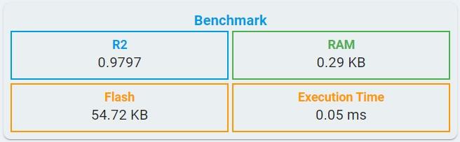
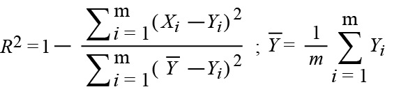
R2: The coefficient of determination. The formula is available in the regression emulation metric section.
FLASH: Minimum flash size required for selected algorithm.
RAM: Minimum RAM size required for selected algorithm.
Execution Time: The estimated time for one inference in the algorithm library, using the LPC55S36 platform (Cortex-M33, 150 MHz, with hard float-point enabled).
Like n-class classification tasks, deep learning models quantify the memory requirements using parameters, such as Algorithm Buffer and Model Size.
Algorithm Validation Results:
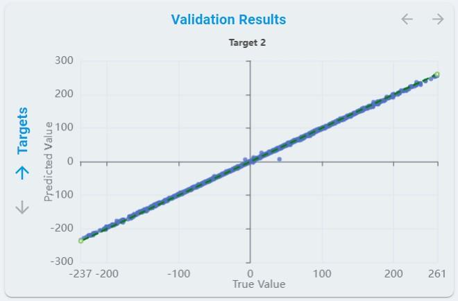
The predicted values of each regression target for all validation sets are plotted for each regression.
The x-axis means the validation sample index.
Train/Val Ratiovalidates the number of samples used for validation.The y-axis means the predicted value.
The dotted line represents the true value.
Evaluation Matrix:
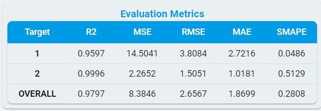
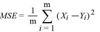
MSE: The mean square error.
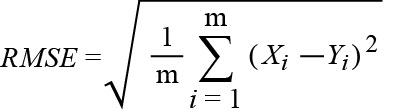
RMSE: The root mean square error.
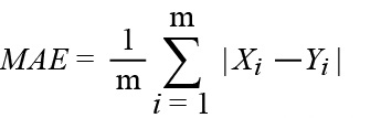
MAE: The mean absolute error.
R2: The coefficient of determination.
SMAPE: The symmetric mean absolute percentage error.
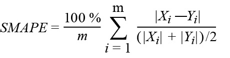
*Notes: In the formulas, Xi is the predicted ith value. The Yi element is the actual ith value. The regression method predicts the Xi element for the corresponding Yi element of the ground truth dataset. Reference comes from [the coefficient of determination R-squared is more informative than SMAPE, MAE, MAPE, MSE, and RMSE in regression analysis evaluation.]
Training Process
This section introduces how to start, pause, stop, and manage training.
Start New Training
Click the Start New Training button.
If this is your first time training, a Training Config pop-up will appear. Please refer to the New Training section below for detailed configuration instructions.
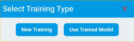
If you already have trained models for your project, a Select Training Type pop-up will appear. It includes two options:
New TrainingUse Trained Model
If you select New Training, the process will be the same as your first-time training. Refer to the New Training section for configuration details.
If you select Use Trained Model, please refer to the Use Trained Model section below for detailed configuration instructions.
New Training
Click New Training button, and a pop-up box appears for configuration. You can rename the training in the Name box. Before you click the Start button, check the feasible options to configure for the different algorithm tasks. Usually, you can go for training without changing the configuration and get the best result.
The following is the configuration option for anomaly detection.
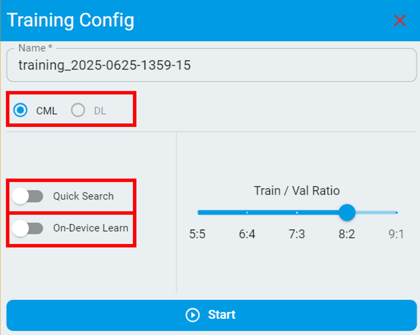
The anomaly detection algorithm is based on semi-supervised machine learning that supports on-device training.
Current only supports
CMLmodels.DLmodels are not enabled.If the algorithm is for prediction only, do not enable
On-Device Learn. This action results in a larger RAM/flash size.If the dataset in use has variations, you can enable
On-Device Learnto allow on-device training.If you want to get training results quickly, enable
Quick Search. The search scope of this mode is not as large as the default mode.
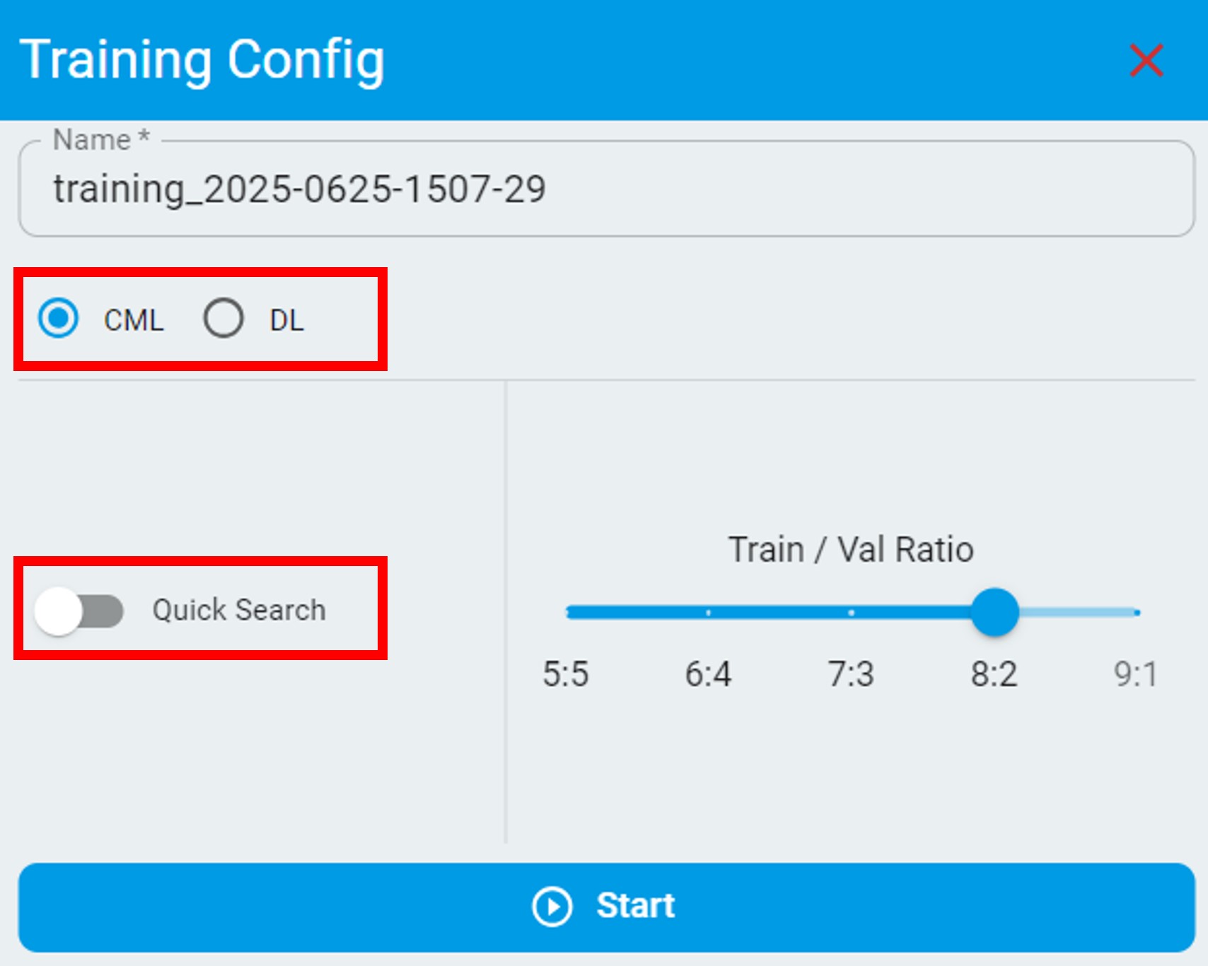
The following are configuration options for classical machine learning in classification and regression tasks:
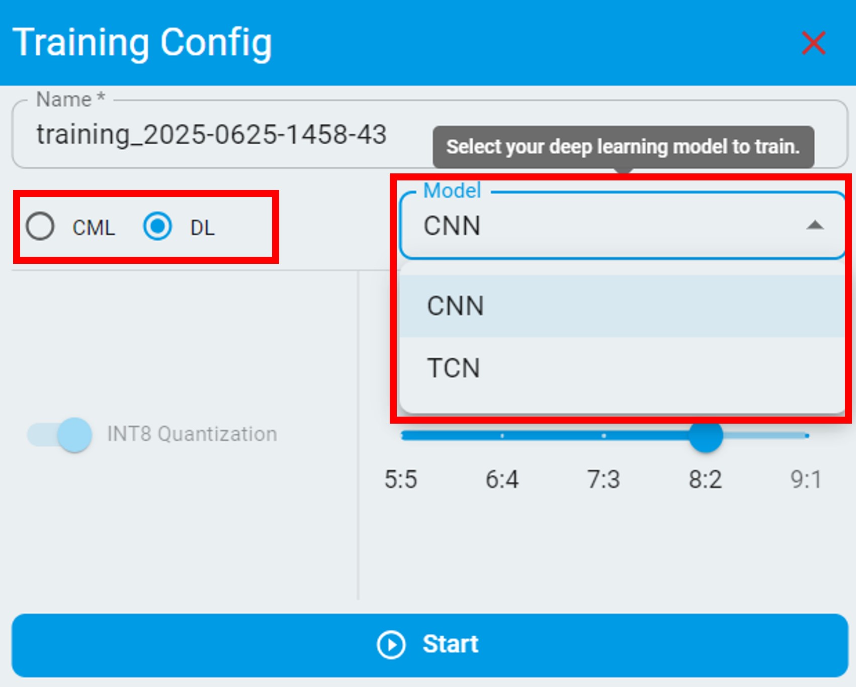
The following are configuration options for deep learning in classification and regression tasks, you can select a specified deep learning model to train:
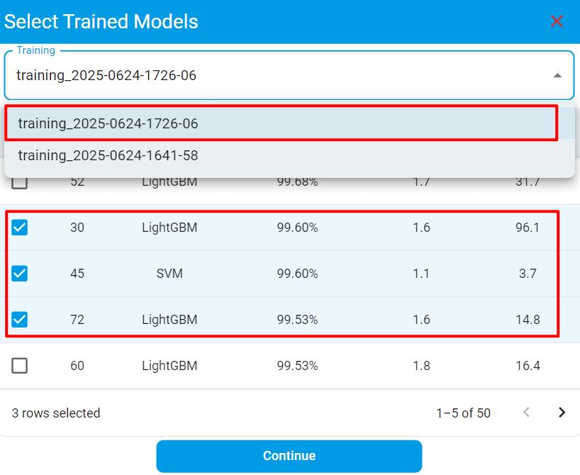
Use Trained Model
When you select the Use Trained Model option, you can start a new training based on previously trained models within your project. Internally, our training engine will parse the selected model(s) and leverage their existing knowledge to build a more specialized model(s) for the new training.
Compared to the New Training option, this approach builds upon prior model knowledge, which can potentially reduce both training time and computational resource usage.
This option is especially useful when you’ve only updated the training dataset since the last training and want to quickly generate new model(s).
Common Options:
Configure
Train/Val Ratio, change with a different ratio if the train/emulation accuracy mismatches or is out of range.
After the training configuration is done or the settings are set to default, click the Start button. Wait until the training is complete. The time to complete the training depends on:
The size of the dataset.
The type of algorithm task you choose.
Different training configurations can also result in different time costs.
If everything is done and a good result has been achieved, read through the results.
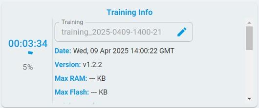
When training starts, the training progress bar is continuously updated, and the timer keeps counting until all content is 100% complete.
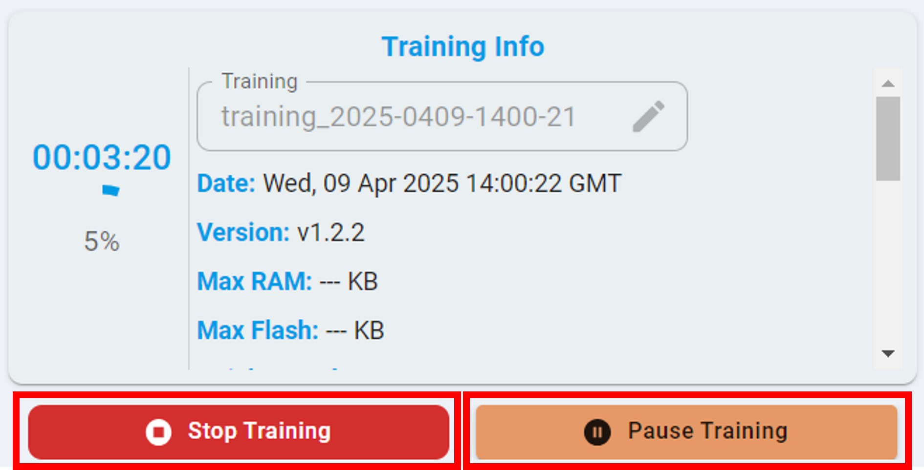
Pause/Stop Training
During the training process, you can choose to click the Stop button to stop the training or click the Pause button to pause the training.
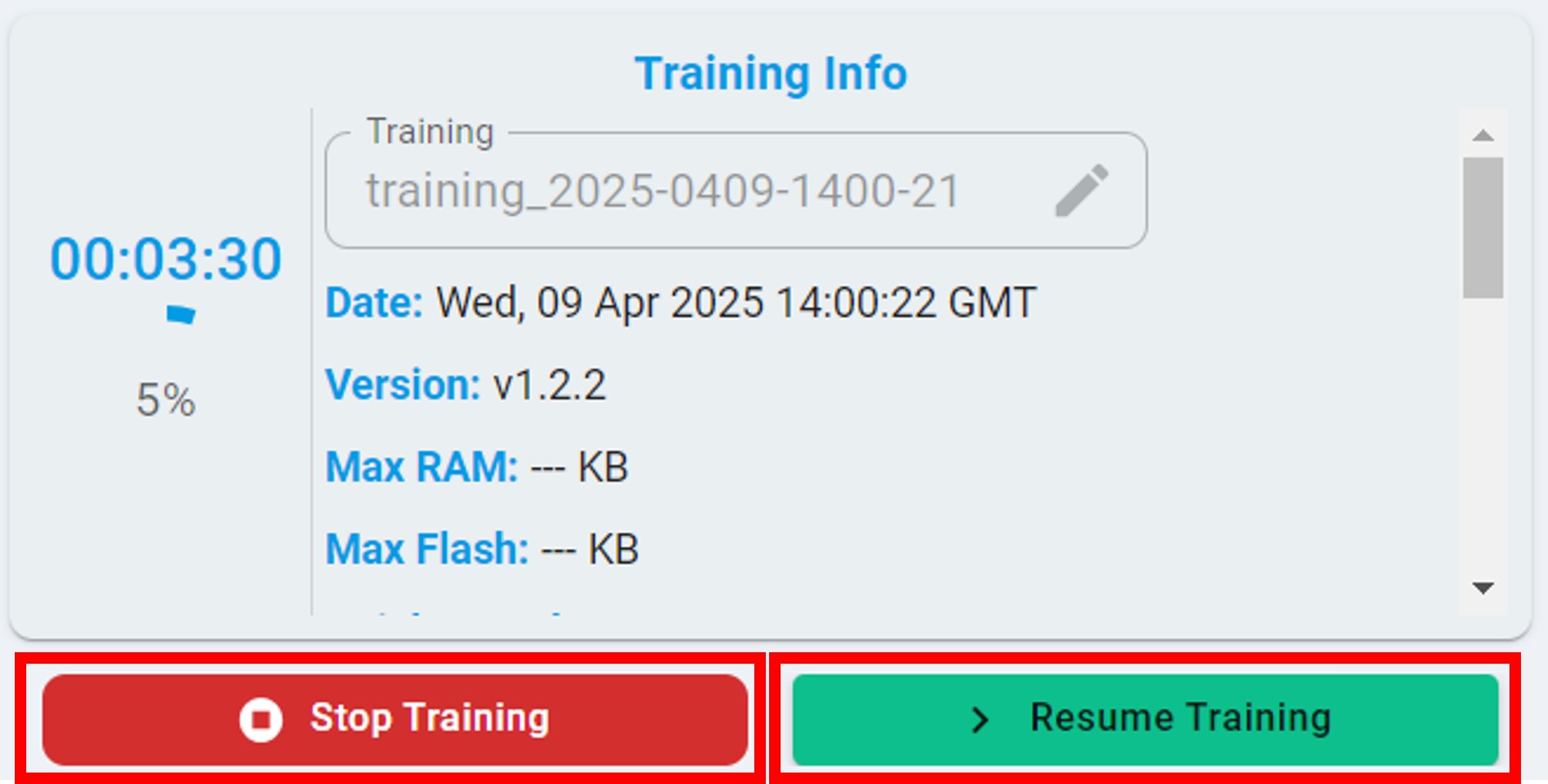
After the pause, you can view the training results of any model in the model list on the left. Alternatively, you can click the Resume button to continue the training.
Training Record Management
As shown in the figure below, after tasks are completed, all training records appear. The candidate algorithm list appears and is sorted by performance.
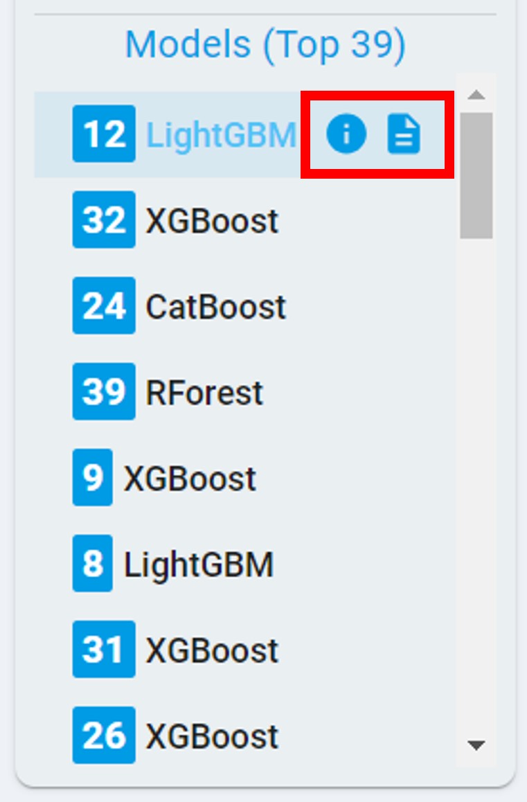
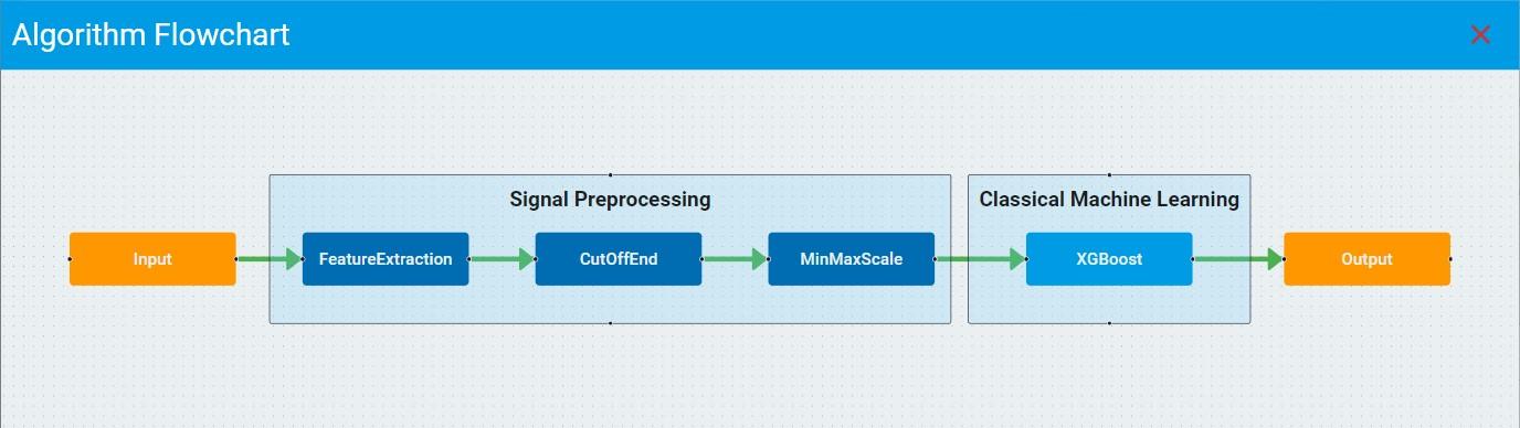
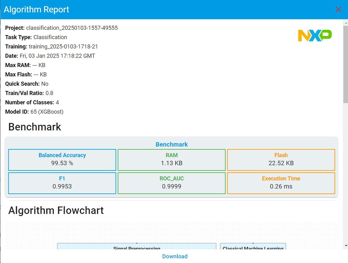
Click the flowchart and report buttons and view/download the flowchart and report of the corresponding model for further references.
Click and choose any of the algorithm results from the list and get the benchmark details as below. In the Training diagram, the purple arrow coordinates indicate the currently selected model. You can also view the auto machine-learning training curve and the balanced accuracy, flash, and RAM corresponding to each model.
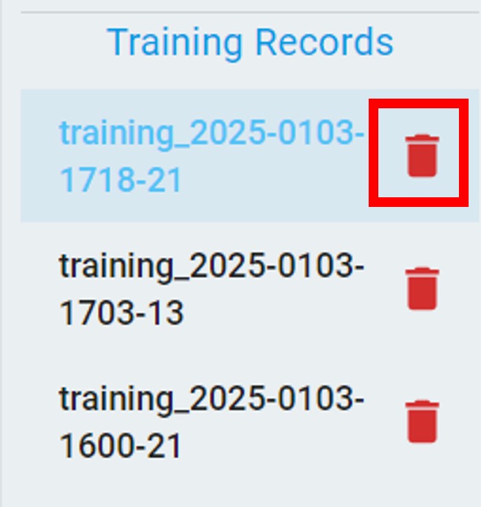
In addition, you can also delete the corresponding training record by clicking the Delete button. After deletion, all model information under the training record will be deleted at the same time.
Model List and Code License
To keep the algorithm transparent as required by customers, we keep the list of all supported models updated according to the release version.
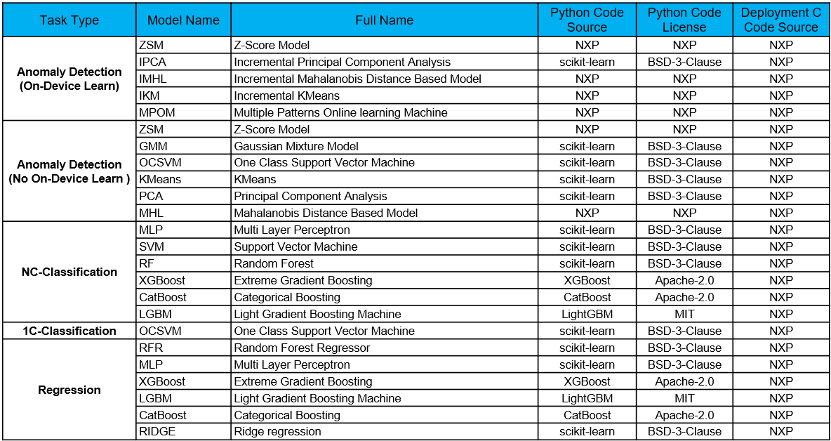
Classical Machine Learning Model List
Deep Learning Model List
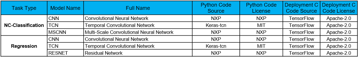
The table highlights the following information:
Models for each task.
Python code source which used for training.
Python code license type.
C code source which used for deployment.
C code license type.