Arc Fault Circuit Interrupter (AFCI) Solution
The Arc Fault Circuit Interrupter (AFCI) is a critical safety device designed to prevent electrical fires by detecting dangerous electrical arcs in home wiring. Unlike traditional circuit breakers, AFCI uses advanced thermal and magnetic mechanisms to offer enhanced protection against overloads and short circuits, significantly reducing fire risks.
The AFCI Solution, developed on TSS, uses machine learning for precise arc detection. It allows users to import raw current data containing arcs, label them using a built-in Data Labeling tool, and automatically generate training datasets. This solution trains and evaluates models to produce deployable algorithm libraries. These libraries integrate seamlessly into electrical systems to ensure robust safety and efficiency.
Create New Project
Navigate to
AFCItask from left menu bar.
Select
Createfrom navigation bar and click theCreate New Projectbutton and create a project.

A navigation bar at the top of the window lets you switch between different operation steps when you click the icons.

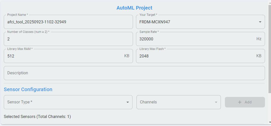
Configure the project settings.
a. Choose the target board. If the list does not include the real board, choose a board with the same CPU.
b. Set the number of classes according to the dataset and your requirements. We use
2classes as an example.c. Set the sample rate of your raw data, all data must have the same sample rate.
d. Set
Library Max RAMandLibrary Max Flashfor the library according to your actual situation.e. Configure the sensor type and the number of channels assigned to each sensor based on the uploaded data. Click the + Add button to save the configuration of the current sensor. In this sample, a Current sensor with 1 channel is used.
f. Confirm completion of the creation. After successful creation, it appears as a working project in the project list.
Data Labeling
The Data Labeling Tool enables users to categorize the imported raw data by applying corresponding tags, such as arc or no-arc, to different sections of the current graph through a visual interface. This tool then segments the raw data based on labels and creates datasets optimized for training machine learning models.
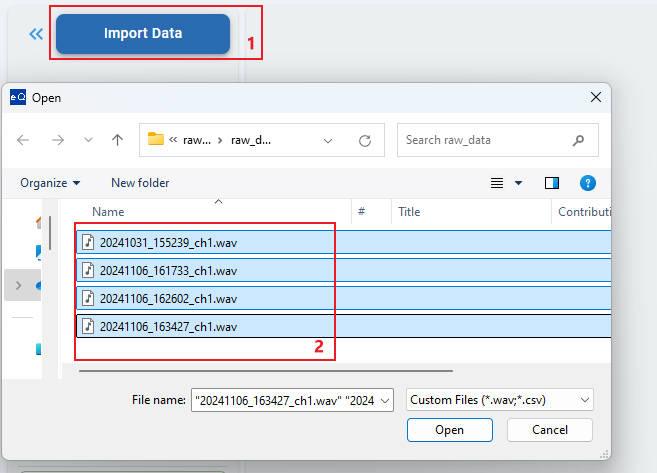
Data Import
AFCI raw data: Continuous current data, stored as a continuous format by time sequence. It is single-channel data, in CSV format (values separated by spaces) or float32 WAV format (single channel).
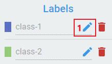
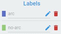
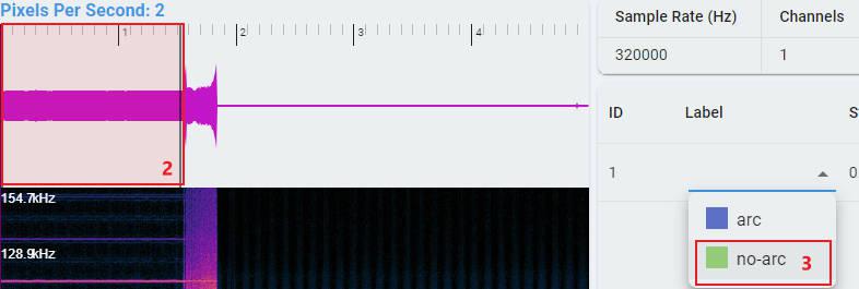
Rename Labels
The label list contains labels for classification. The number of labels in the list corresponds to the number of classes.
By default, the label of the class is a class index. You can edit the alias of the class to create a label for the class (optional).
You can edit the alias of labels. This operation is optional and only intends to enhance the label readability.
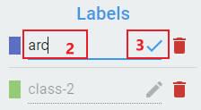
To edit the alias, first click the edit button:
Second, input the alias string, then lick the check button to apply the rename.
To rename all labels one by one, repeat the above steps.
Labeling Operations
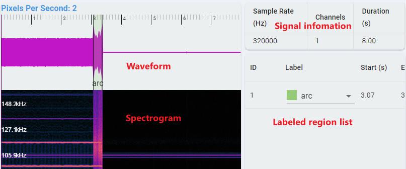
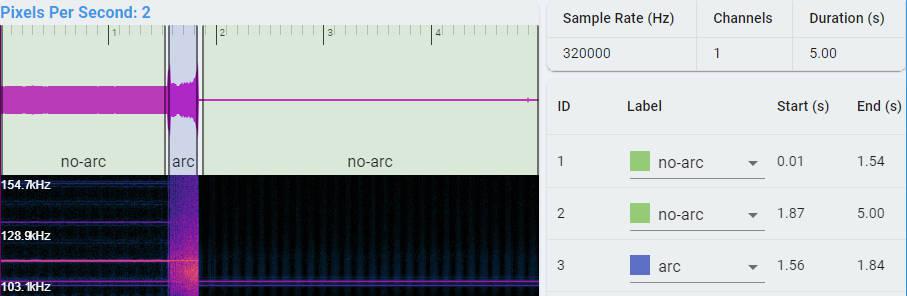
Waveform: Time series waveform of data.
Spectrogram: Time-frequency domain waveform of data, using STFT transform, the abscissa is time, the ordinate is frequency.
Labeled region list: Each region drawn on the time series waveform corresponds to a record here, including the classification label, start time, end time.
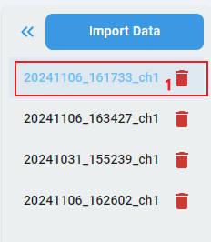
Step 1: Select a file in the file list to label.
Step 2: Draw a range on a waveform graph.
Step 3: Choose the label for the labeled region.
Repeat steps from 2 to 3 and label all the regions.
Repeat steps from 1 to 3 and label all the regions.
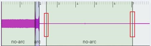
Edit Labeled Result
You can modify the range of a region by dragging its boundaries. You can modify the label of region by selecting the label.
Segment
Segment is a tool that processes raw data by saving the corresponding data or each region as separate files based on the labeling results. Then, it converts these files into a classification data format suitable for model training, including a train/test split. Finally, it imports the data into the project dataset, allowing you to view the classified data on the dataset page.
You can get the suggested value of Window Size, Stride, Frequency by clicking the Start Analysis button (calculated by the Data Intelligence).
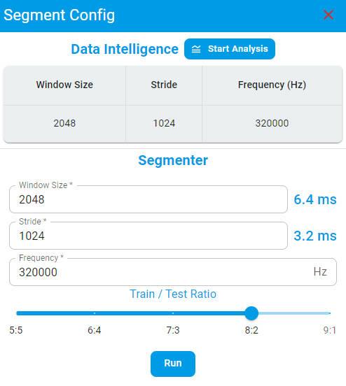
Window Size — Window size of the training data, the left side is the corresponding time duration.
Stride — The step size of sample windows generation, defines how much forward movement occurs relative to the previous window when extracting a new window from continuous data, which directly impacts the overlap between adjacent windows.
Train/Test Ratio — The ratio of training and test data.
After completing the settings, click the Generate Dataset button and wait. The system redirects to the dataset page with all labeled data imported, allowing you to start training immediately.
Note:
All ranges must be labeled before running the Segment.
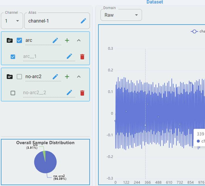
Dataset
All training data generated by Segment from Data Labeling have been automatically imported. You can view the distributions of the dataset across different domains on this page as visual graphs, or you can choose not to act.
Data feature chart can be viewed with single file or multiple files in different domains. This feature can facilitate users to analyze and compare intuitively.
* Raw domain with Combined and Separated modes.
* Temporal domain with the ACF and the PACF operators.
* Statistical domain with the Min, Max, Mean, Mean_Plus_STD and Mean_Minus_STD operators.
* Spectral domain with the FFT, STFT and Cepstrum operators.
For more detailed information, refer to Dataset.
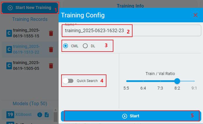
Training
Clicking the Training icon in the navigation bar redirects you to the Training page.
Click the
Start New Trainingbutton and enter into theTraining Configstage.The alias of the training can be edited (optional).
Choose CML or DL models.
If the
Quick Searchbutton is toggled, the training process can be finished in a relatively short time, while the training performance may not be the best (optional).Click
Startand start the training.
For more detailed information, refer to Training.
Emulation
After training is finished, Clicking the Emulation icon on the navigation bar redirects you to the Emulation page.
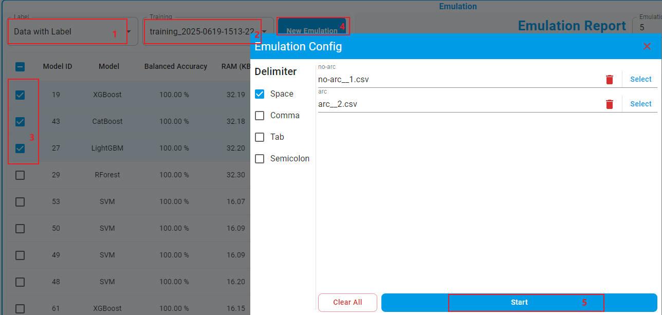
Data with Label
Choose
Data with Label.Choose your training record from the drop-down menu. The trained models are shown in detail in the table.
Choose the models to be emulated.
Click the
New Emulationbutton, the test dataset generated by Segment of Data Labeling is selected automatically.Start the emulation, and check the real accuracy.
Reports are generated for each emulated model.
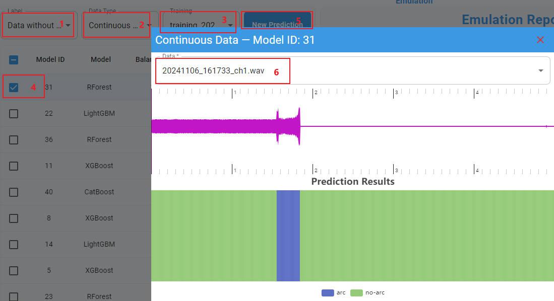
Continuous Data without Label
Choose
Data without Label.Choose
Continuous Data.Choose your training record from the drop-down menu. The trained models are shown in detail in the table.
Choose a model to prediction.
Click the
New Predictionbutton.Select a raw continuous data in the data list (must be imported in the Data Labeling).
The continuous signal waveforms and the prediction results are displayed in the graphs.
For more detailed information, refer to Emulation.
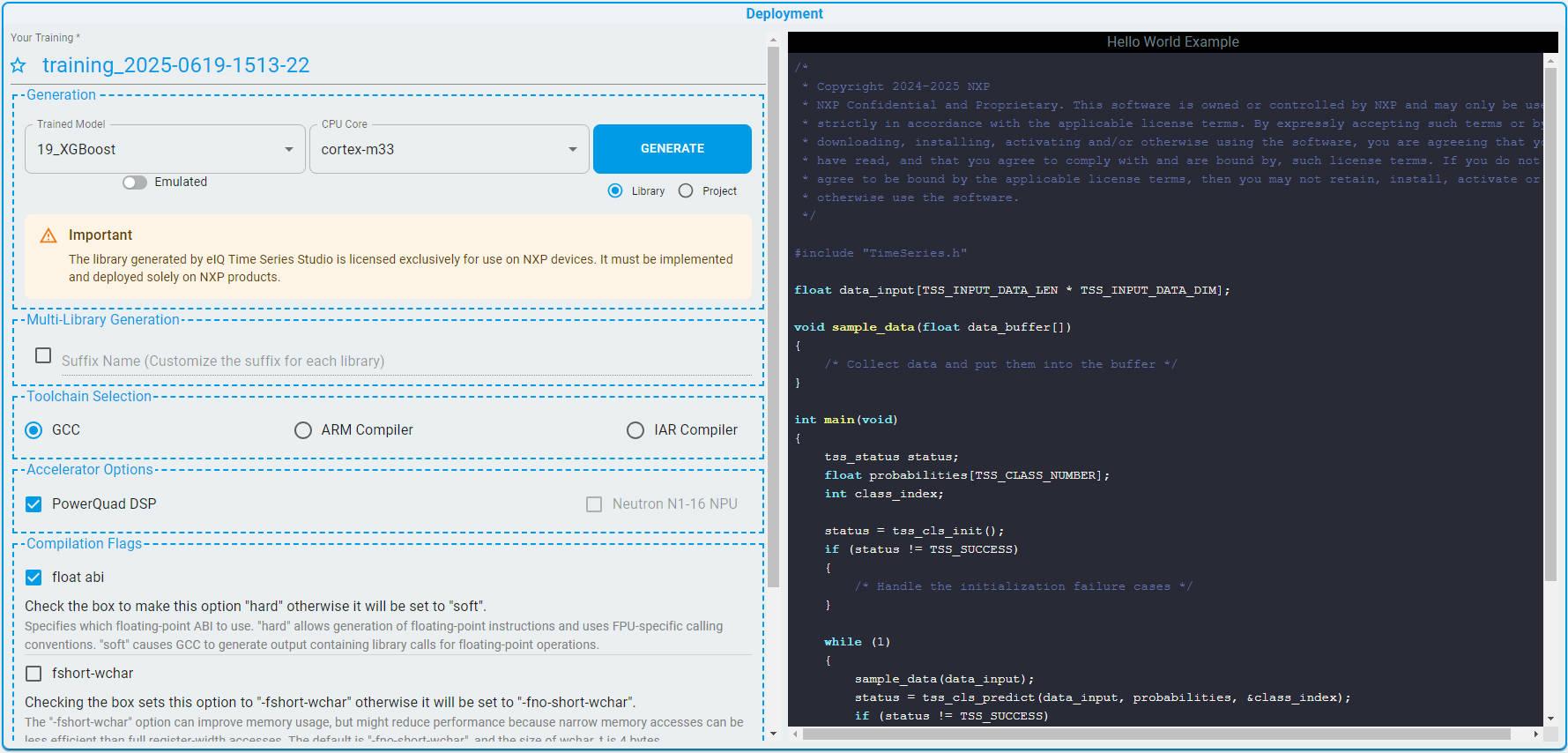
Deploy To Device
Choose your model.
Configure the compilation options based on the actual situations.
Click the
GENERATEbutton and save the algorithm library.Refer to the example code and deploy the library to your device. If using the MCUXpresso IDE, you can also choose to generate a sample project.
For more detailed information, refer to Deployment.